Introduction

MRI is an indispensable tool for non-invasive detection of neuropathology. The unparalleled rich tissue contrasts it provides, however, are mostly indirect measurements of tissue properties and lack specificity compared to histology. In this work, we investigated whether deep learning can generate MRI-based contrasts to match the contrasts of several histological methods. We have developed a series of deep learning networks, called MRHNet, based on the carefully curated histological data from the Allen mouse brain atlas¹ and co-registered high-resolution MRI data. The MRI data consisted mainly of a large set of diffusion MRI (dMRI) data, which offer several tissue contrasts linked to tissue microstructure. The results were validated using test data from normal and genetically modified mouse brains. We further sought to understand the inner-working on the network and used the network to evaluate the contribution of individual image.

Materials & Methods

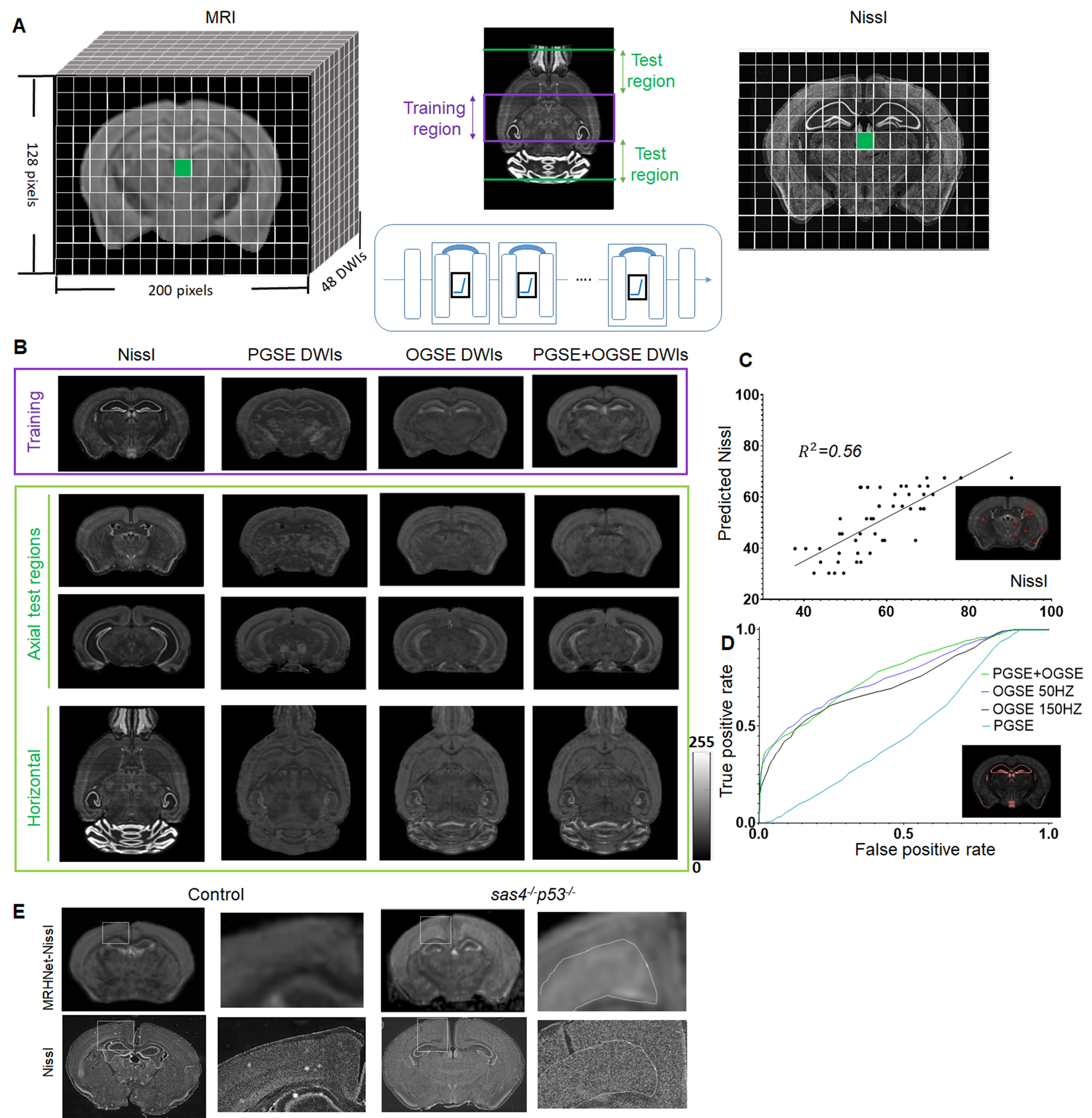
A series of deep learning networks, called MRHNet, were constructed to take multi-contrast MRI data (mostly ex vivo mouse brain dMRI data, C57BL/6, n=12) as inputs and co-registered histological images from the Allen Brain Atlas (ABA) as the target (Fig. 1A), including Nissl/Neurofilament/MBP (for neuronal/axonal/myelin structures) as the target. We used data from part of the forebrain region for training and the rests for testing. For further validation, we acquired data from the Sas4^-/-p53^-/- mouse brains, which had abnormal cortical cell masses², and litter-mate controls (n=4/4) and the shiverer mouse brains, which showed dysmyelination³, and controls (n=4/4). Ex vivo dMRI data were acquired with 30-60 directions, b-value of 700-5000 s/mm², both oscillating (OGSE, 50-150 Hz) and pulsed gradients (PGSE, Δ=15ms)⁴, and a resolution of 0.1x0.1x0.1 mm³ to match the ABA data. A 5X5 patch size was used to accommodate residual mismatches between histology and MRI data. Approximately 40,000 such 5X5 patches were used to train the network.

Results

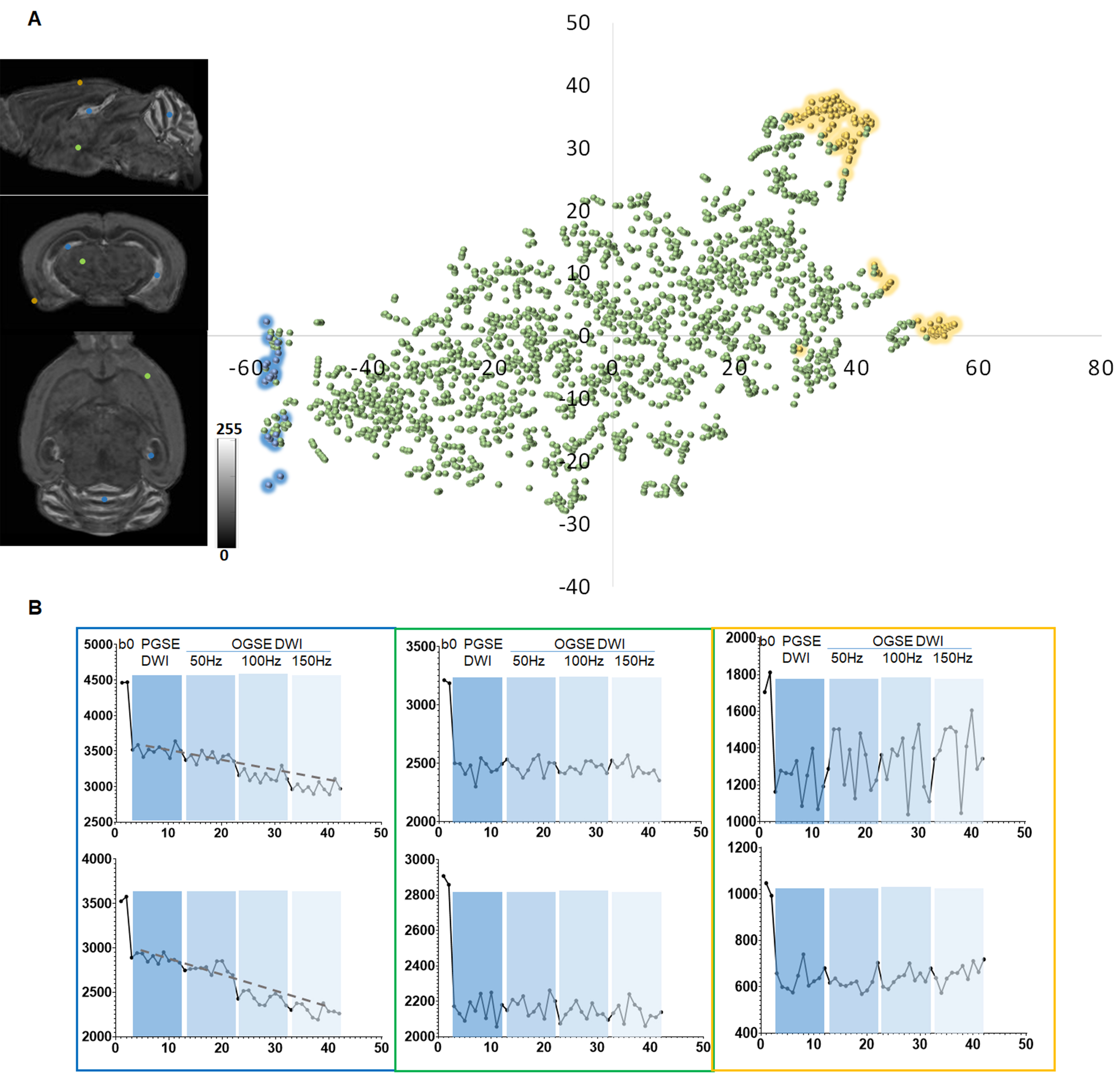
We first tested whether MRHNet trained using Nissl data can generate contrasts that resembled the tissue contrasts in Nissl stained sections. In the testing regions, the network that utilized all OGSE and PGSE dMRI data as inputs generated MRHNet-Nissl maps with good agreement with the ground truth Nissl data (Fig. 1B-C), with higher sensitivity and specificity than results with partial data (Fig. 1B-D). The MRHNet-Nissl map of the Sas4^-/-p53^-/- mouse brains produced image contrasts that closely matched Nissl-stained histology.

We then used the t-Distributed Stochastic Neighbor Embedding (t-SNE)⁵ to visualize the feature space to better understand the inner-working of MRHNet. In Fig. 2A, a majority of the patches corresponded to regions with low Nissl signals, whereas patches in the lower-left corner corresponded to regions with strong Nissl signals and several patches on the upper-right corner corresponded to the brain surface. Fig. 2B shows representative signal profiles from the three categories. Patches that corresponded to strong Nissl signal regions showed decreased signals as the oscillating frequency increased, whereas the other two types of patches show no such pattern.

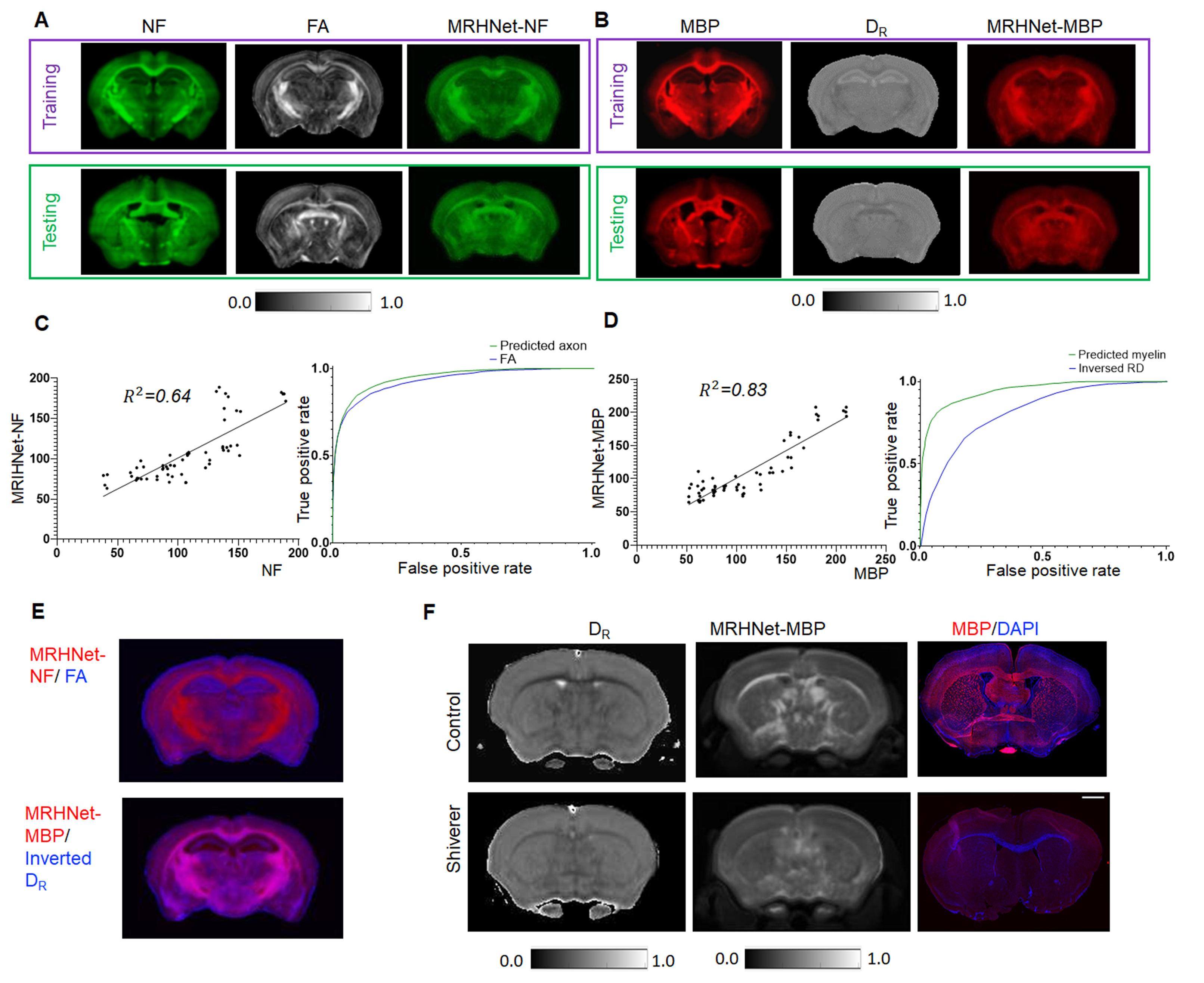
We also trained networks using axon and myelin stained histology (Fig. 3A-B), and both showed improved sensitivity and specificity than commonly used fractional anisotropy (FA) and radial diffusivity (D_R), as shown by the ROC analysis (Fig. 3C-D) and regional difference maps (Fig. 3E). In Fig. 3F, MRHNet-MBP map based on dMRI data from the dysmyelinated shiverer mouse brain suggested reduced myelin than controls.

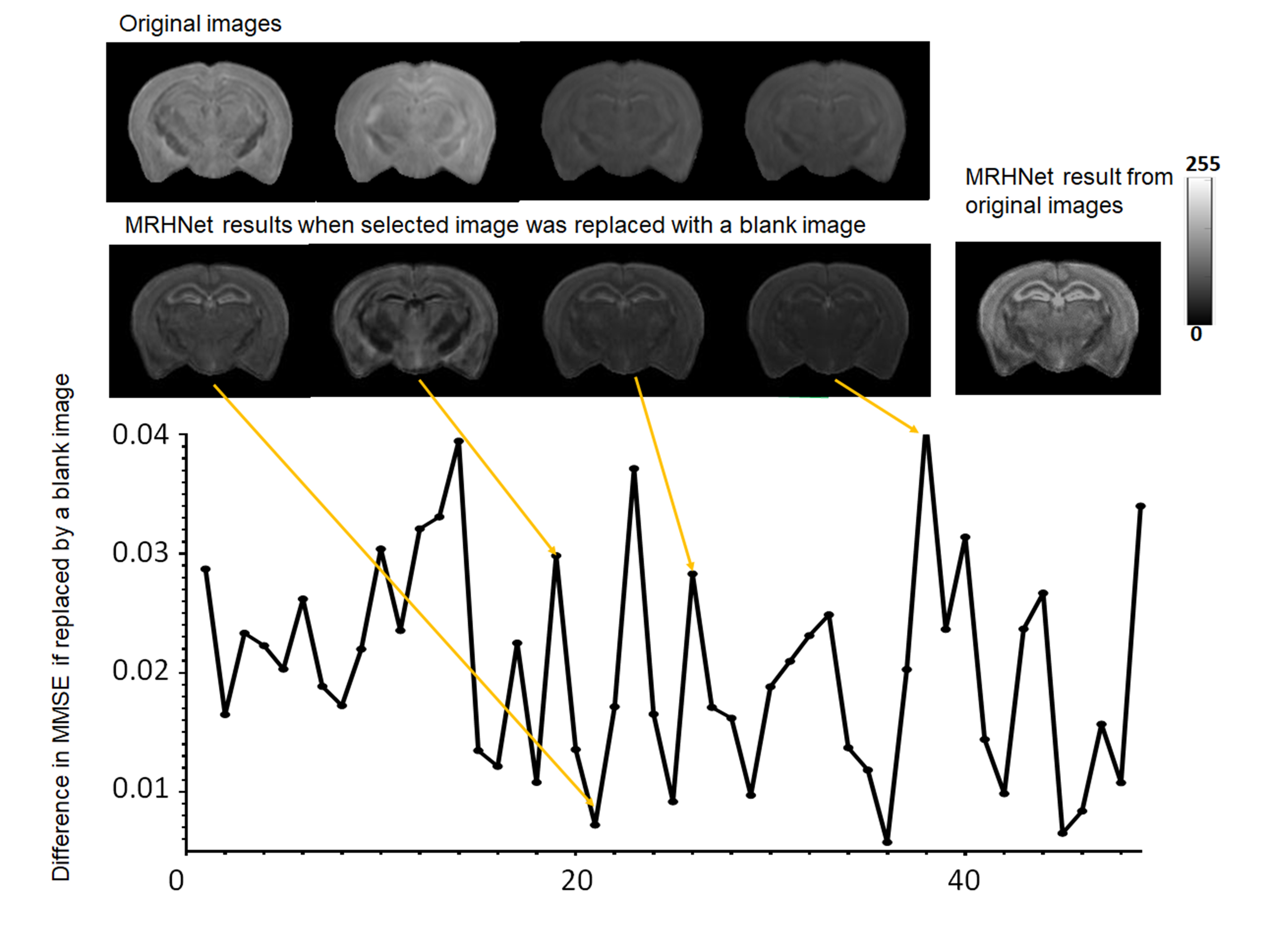
We further analyzed the contribution of each dMRI data to the network outcomes by replacing the individual image with an image with constant signals and measured the RMSE of the results compared to the ground truth (Fig. 4). We found that the contribution of individual dMRI data were unevenly distributed.

Discussions

Our results demonstrate that deep learning can assist the development of highly specific markers from MRI data. While significant correlations between several dMRI-based markers and histological measurements of axon and myelin have been reported, the proposed network can potentially generate the optimal markers for the given MRI data. The co-registered MRI and histological data enabled us to validate the sensitivity and specificity of these markers. The technique may assist the development of optimal multi-contrast MRI and new MRI contrasts by quantifying the contribution of individual image to detect certain histopathological features.

Our study is not without its limitations: 1) the MRI and histology data used in this study were acquired from different mouse brains of the same strain; 2) the networks were based on ex vivo mouse data and may not apply to in vivo data due to the differences between in vivo and ex vivo MRI signals; 3) the resolution of MRI remains limited compared to histological data; and most importantly, 4) data from cases with complex neuropathology, e.g., inflammation and edema, are not present in the training dataset, which may limit the applicability of the technique for such cases.

Conclusion

Our results demonstrate that deep learning based on co-registered MRI and histological data can improve the sensitivity and specificity of MRI in detecting certain histopathological features in the brain.

Acknowledgements

This study was supported by NIH R01NS102904