Introduction

Arterial spin labeling (ASL) MRI techniques provide cerebral blood flow (CBF) measures without the use of contrast agent. It has provided largely consistent results with DSC perfusion MRI in delineating hypoperfused regions in arterial ischemic stroke (AIS)^{1, 2}. However, the precise delineation of hypoperfusion lesion and penumbra in ASL images remains challenging due to the low SNR and delayed arterial transit. Deep learning (DL), an advanced Machine Learning (ML) method, captures the hierarchical features of the input image automatically and can identify, classify, and quantify patterns in medical images^{3, 4}. In this study, we developed and evaluated a DL-based algorithm to automatically identify the hypoperfusion lesion and penumbra in ASL images using the lesions from DSC MRI as supervision.

Methods

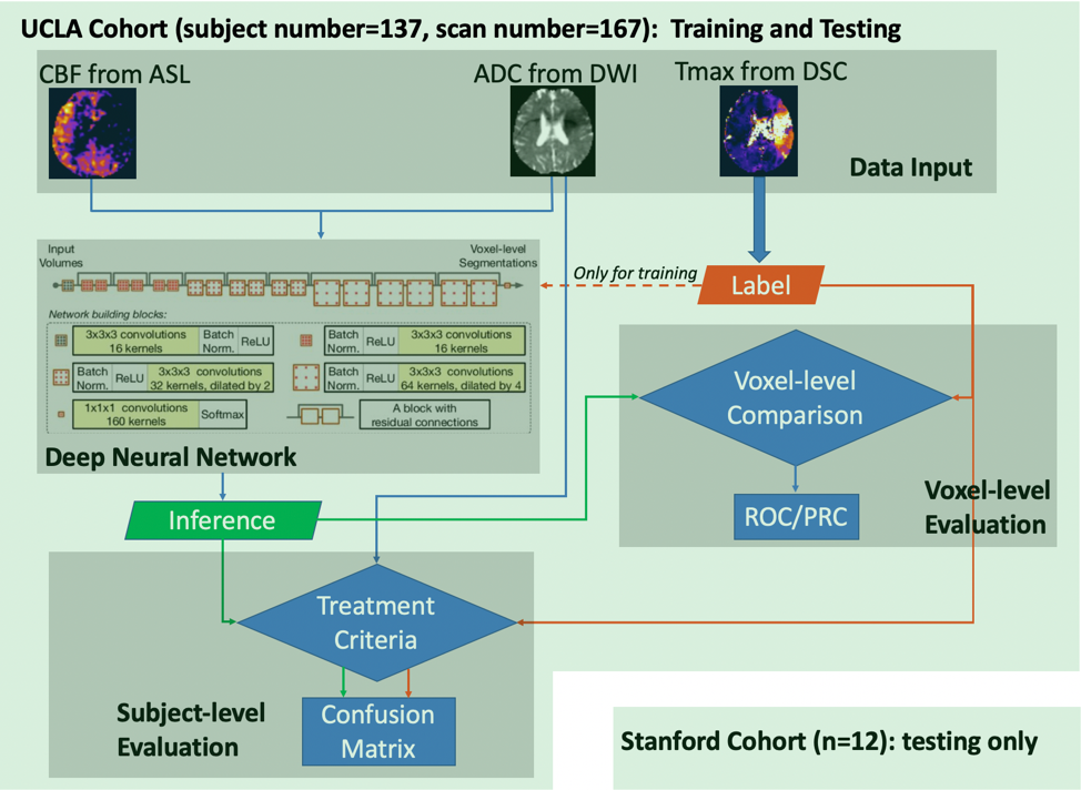
The flowchart of the DL algorithm deployment is shown in Figure 1, including modules of data input, DL model architecture, voxel-level and subject-level evaluation. The following describes each step in detail.
1. Data Acquisition and Processing
The study included MRI data from two AIS cohorts: 167 image sets from 137 patients scanned on Siemens 1.5T Avanto or a 3T Tim Trio systems at UCLA (1.5T: n=93; 3T: n=74), using 3D GRASE pCASL with PLD of 2000ms; and 12 MRI from 12 patients scanned on GE 1.5T and 3.0T SIGNA systems at Stanford University (1.5T: n=1; 3T: n=11), using 3D pCASL with fast spin echo and stack-of-spirals readout trajectory and PLD of 2000ms. DSC images were acquired using a gradient-echo EPI sequence, and the Time-to-Maximum of the residue function (Tmax) map was generated using a cSVD method by the commercial software OLEA (La Ciotat, France) for the UCLA cohort. The RAPID software (iSchemaView Inc, Menlo Park, CA) was used for analyzing DSC data from the Stanford cohort. Following skull-stripping, brain segmentation, manual masking and thresholding by 6sec^5-7, Tmax labels were generated from Tmax maps.
2. Network and Training
The HighRes3Dnet⁸ with 20 layers and residual connections was trained on 2 Nvidia GeForce GTX 1080 Ti GPUs via NiftyNet⁹. CBF and ADC images were used as input, and the Tmax label image served as the supervision. 48*48*48 volumes (batch size=4) were randomly extracted from 3D preprocessed images for training. Volume-level augmentation was employed including rotation and random spatial rescaling. The training process was performed with 70,000 iterations, with Dice loss and Adam optimizer (learning rate = 0.0001, β₁=0.9, β₂=0.999). Ten-fold cross-validation was used so that the whole dataset can be evaluated for inference performance.
3. Machine Learning Models and Training
For comparison, six commonly used ML classifiers were trained on the same UCLA cohort, including linear regression classifier, ridge regression classifier, kernel ridge regression classifier, neural network classifier, Support Vector Machine (SVM) with Radial Basis Function (RBF) and random forest classifier¹⁰. The same 10-fold cross-validation scheme as used in the training of the DL model was applied.
4. Model Performance Assessment
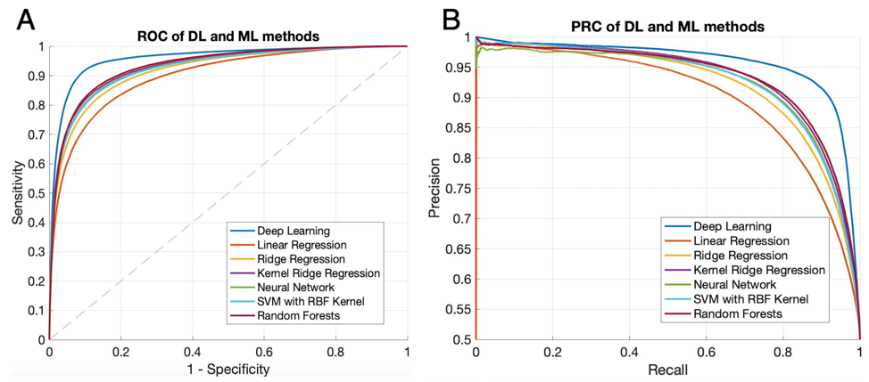
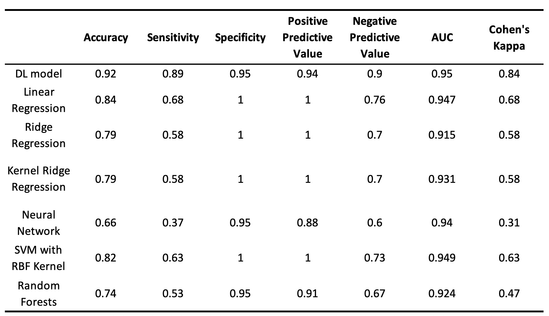
The DL model performance was evaluated on a subset of the UCLA cohort who met the inclusion criteria for DEFUSE 3 trial⁵. For voxel-level evaluation, the group average Dice between the inference and the Tmax label was calculated as the average of Dice coefficient of all subjects. The Receiver Operating Characteristic (ROC) curves and Precision-Recall (PR) curves were calculated. Subject-level performance was based on the criteria of perfusion/diffusion mismatch by the DEFUSE3 trial⁵. Confusion matrices, sensitivity, specificity, positive predictive value (PPV), negative predictive value (NPV), the total accuracy, and Cohen’s kappa coefficient were also calculated¹¹ for the DL and 6 ML models, respectively.

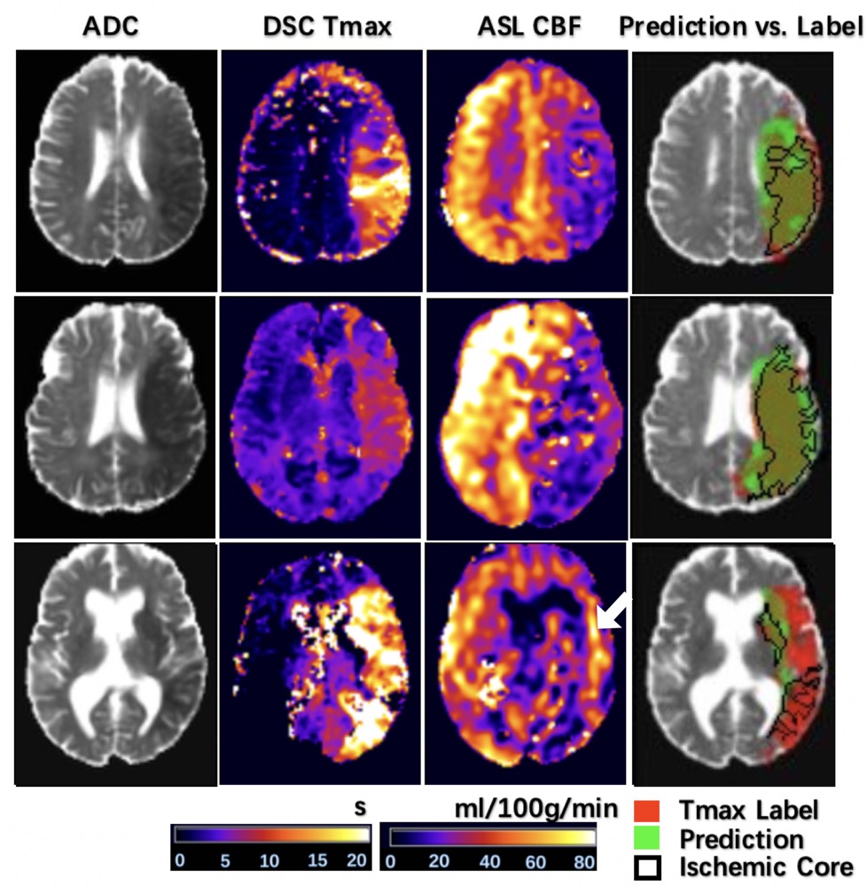
Results and Discussion

Figure 2 shows 4 representative cases at 1.5T and at 3T from the UCLA cohort, respectively. Only the second case of 1.5T was misclassified. Overall, the network could identify the perfusion lesion defined by Tmax images although there were discrepancies between the lesion volumes of ASL and DSC MRI. The group average Dice coefficient was 0.47±0.23. The ROC and PR curves showed our DL model achieved significantly superior performance compared to traditional ML methods (p<0.001). The AUC of the ROC and PR curve for our DL model was 0.958(Figure 3A) and 0.957 (Figure 3B). For endovascular treatment eligibility, Figure 4 shows that the accuracy, sensitivity, specificity, PPV, NPV, and Cohen’s kappa coefficient of our DL model were systematically superior than ML models. The overall accuracy was 0.92 (95% CI: [0.79, 0.98]).
Our pretrained DL models were tested on the 12 ASL datasets of the Stanford cohort, without any fine-tuning of parameters. Three cases are shown in Figure 5. The average Dice coefficient was 0.43±0.25. Voxel-level evaluation showed that the AUC of the ROC and PR curve was 0.942 and 0.931, respectively. Subject-level evaluation yielded an accuracy of 0.92 (95% CI: [0.62, 0.99]), with sensitivity, specificity, PPV, and NPV of 0.75, 1.00, 1.00 and 0.89, respectively.

Conclusion

With a high accuracy of 92% for imaging-based criteria for endovascular treatment in two independent cohorts of AIS patients and superior performance compared to ML methods, the proposed ASL perfusion DL model provides a promising approach for assisting decision-making for endovascular treatment in AIS patients.

Acknowledgements

The authors thank Drs. Yonggang Shi and Ben Duffy for helpful discussions. This work was supported by National Institute of Health (NIH) grants UH2-NS100614, R01EB028297, R01NS066506.