1270
Implementation of Low-cost FPGA-based Magnetic Particle Imaging System
Congcong Liu1,2, Caiyun Shi1, Jianguo Cui2, Xin Liu1, Hairong Zheng1, Dong Liang1, and Haifeng Wang1
1Shenzhen Institutes of Advanced Technology,Chinese Academy of Sciences, Shenzhen, China, 2Chongqing University of Technology, Chongqing, China
1Shenzhen Institutes of Advanced Technology,Chinese Academy of Sciences, Shenzhen, China, 2Chongqing University of Technology, Chongqing, China
Synopsis
Conventional Magnetic Particle Imaging (MPI) systems are expensive and bulky, and most of them use CPU and MPU as controllers. Field Programmable Gate Arrays (FPGAs) have recently become widely utilized as controllers in many systems for flexibility and speed. In this paper, we proposed an implementation scheme of a low-cost, small-volume MPI system based on FPGA architecture. The experimental results showed that the complete operation of the MPI system signal link could be realized by the low-cost FPGA-based control system (≤$200), and the distribution of the superparamagnetic iron oxide nanoparticles (SPION) could be imaged by the signal of the particle.
Introduction
Recently, MRI systems have been developped from high-cost and large-size toward low cost and portability 1,2. As a promising imaging method, most of Magnetic Partial Imaging (MPI) systems also have high-cost, limited-configuration and large-size3-7. Recently, MPI systems have evolved toward low cost, flexibility and portability7-10. However, hundreds of thousands of dollars of external support devices are deployed in such systems, and these devices also increase the size of the system. In this paper, an MPI system solution based on the Xilinx ZYNQ 7010 console (≤$200) was implemented, which has the advantages of low cost, flexibility and small volume. The signal generator and data acquisition card were replaced by the Field Programmable Gate Arrays (FPGAs) board to realize generation of excitation signals and the acquisition and transmission of superparamagnetic iron oxide nanoparticles (SPION) signals, thereby making the system more integrated and less expensive(≤$7000). In the actual experiments, the feasibility of the system has been validated by calculating and imaging the distribution of the particles by the SPION signals.Methods
MPI systems typically consist of a main magnet, an excitation coil, and peripheral support hardware circuitry11-14. The FPGA controller used in this system is a commercial dedicated high-speed signal processor based on the Xilinx ZYNQ 7010 Soc, which costs only $164. The DDS technique with a synthetic excitation signal is adopted in the system. A sampling rate of 125 Msps, 8-bit resolution DACs are connected to receive digital signals from the DDS. In addition to the FPGA system of the ZYNQ 7010 also features a Dual-Core ARM9 CPU running at a clock speed of 667MHz with an embedded Linux OS. The acquisition of the particle signal was executed using an ARM CPU through ADC with a sampling rate of 32 MHz and resolution of 8-bit. The data obtained in ADC is transmitted to the ARM CPU through DMA. Gigabit Ethernet communication scheme based UDP packets is adopted in this system for data communication with the terminal computer.The NdFeB material was adopted to manufacture a cylindrical permanent magnet that forms a gradient magnetic field in the MPI system. A gradient magnetic field of 1.77 T/m could be produced by a permanent magnet with the height of 20 mm and the length of 140 mm on the intermediate plane perpendicular to the central axis. The Litz wire with an outer diameter of 5 mm was selected to produce an excitation coil with a length of 100 mm and a thickness of 20 mm (as seen as Figure 1). When the coil was energized with a single-peak current of 40 A, a maximum excitation magnetic field of 18 mT was generated. Therefore, the range of the FOV was designed to be 20 mm. Here, the proposed system apply a commercial Synomag tracer (as seen as Figure 2(a)) with a particle size of 50 nm and a concentration of 25 mg/ml produced by Micromod Partikeltechnologie GmbH in Germany. Asymmetrical cancellation forms of the custom-made receive coil (as seen as Figure 2(b)) were employed. Experiments were carried out by using a rubber tube and 10ul of SPION to make a phantom (as seen as Figure 2(c)). The experiments were carried out by using a phantom made of a rubber tube and 10ul of SPION.
The form of FFP movement is as follows :
$$\gamma\sin(wt)=x ,(1)$$
Where $$$\gamma=10mm$$$ denotes the boundary value of the FFP from the midpoint of the FOV and $$$w=2\pi f_{0}$$$ represents the angular frequency of the excitation field with $$$f_{0}=20KHz$$$. The distance of the phantom from the midpoint of the FOV is indicated by $$$x$$$. The process of is as follows:
$$t=\frac{b-a-\frac{c-a}{2}}{2}\times\frac{1}{f_{s}},(2)$$
where a, b and c represent the current number of point and $$$f_{s}=32MHz$$$ is the sampling rate of the ADC. The distribution of the SPION particles can be imaged, according to Eq. (1) and Eq. (2).
Results
The experimental results of the proposed low-cost MPI system (as seen as Figure 1) have been demonstrated (as seen as Figure 3 and 4). The phase shift between the three points a, b and c was calculated by the Eq. (1) and Eq. (2) (as seen as Figure 4(a) and (c)) to obtain the offset distance of the particles, which is then compared with the physical offset distance (as seen as Figure 3). The result of the calculation was consistent with the position of the object (as seen as in Figure 5) when the phantom was moved to the midpoint of the FOV. However, when the actual phantom had 3 mm offset to the FOV midpoint, there was an error of 1 mm between the calculated results and the actual offset results (as seen as Figure 5).Conclusion and Discussion
In sum, a low-cost, FPGA-based console-based MPI system has been developed to detect the SPIONs’ signal, which can image the distribution of the SPIONs using the calculated offset position of the particles. The FPGA-based console system costs less than $200, and the entire system costs less than $7,000. The complexity and cost of the entire system is reduced by the integrated FPGA-based controller. In the future, the entire system will be further perfected for more 2D and 3D MPI methods.Acknowledgements
Congcong Liu and Caiyun Shi contributed equally to this work. Thank Prof. Wenzhong Liu from Huazhong University of Science and Technology for his guidance and helps. This work was partially supported by the National Natural Science Foundation of China (61871373 and 81729003), the Strategic Priority Research Program of Chinese Academy of Sciences (XDB25000000), the Natural Science Foundation of Guangdong Province (2018A0303130132) and the Shenzhen Key Laboratory of Ultrasound Imaging and Therapy (ZDSYS20180206180631473).References
- Cooley C Z, Stockmann J P, Witzel T, et al. Design and implementation of a low-cost, tabletop MRI scanner for education and research prototyping. Journal of Magnetic Resonance.2019;106625.
- Anand S, Stockmann J P, Wald L L, et al. A low‐cost (< $500 USD) FPGA‐based console capable of real‐time control. Proc ISMRM. 2018;26:948.
- Gleich B, Weizenecker J. Tomographic imaging using the nonlinear response of magnetic particles. Nature. 2005;435(7046):1214.
- Weizenecker J, Gleich B, Borgert J. Magnetic particle imaging using a field free line. Applied Physics. 2008;41(10):105009.
- Goodwill P W, Conolly S M. Multidimensional x-space magnetic particle imaging. IEEE transactions on medical imaging. 2011;30(9):1581-1590.
- Pi S, Liu W, Jiang T. Real-time and quantitative isotropic spatial resolution susceptibility imaging for magnetic nanoparticles. Measurement Science and Technology. 2018;29(3):035402.
- M.Graeser, F.Thieben, P.Szwargulski, et al. Human-sized magnetic particle imaging for brain applications. Nature communication. 2019;10:1-9.
- Yu E Y, Bishop M, Zheng B, et al. Magnetic particle imaging: a novel in vivo imaging platform for cancer detection. Nano letters. 2017;17(3):1648-1654.
- Weizenecker J, Gleich B, Rahmer J, et al. Three-dimensional real-time in vivo magnetic particle imaging. Physics in Medicine & Biology. 2009;54(5):L1.
- Ferguson R M, Minard K R, Krishnan K M. Optimization of nanoparticle core size for magnetic particle imaging. Journal of magnetism and magnetic materials. 2009;321(10):1548-1551.
- Weizenecker J, Borgert J, Gleich B. A simulation study on the resolution and sensitivity of magnetic particle imaging. Physics in Medicine & Biology. 2007;52(21):6363.
- Goodwill P W, Scott G C, Stang P P, et al. Narrowband magnetic particle imaging. IEEE transactions on medical imaging. 2009;28(8):1231-1237.
- Cooley C Z, Mandeville J B, Mason E E, et al. Rodent cerebral blood volume (cbv) changes during hypercapnia observed using magnetic particle imaging (mpi) detection. NeuroImage. 2018;178:713-720.
- Liu C, Cui J, Li N, et al. Preliminary Study of Gradient Coils with Variable Gradient Valueand Open-Drive Coil in Magnetic Particle Imaging. Proc. IEEE RCAR, Irkutsk, Russia, August 2019;171:958-963.
Figures
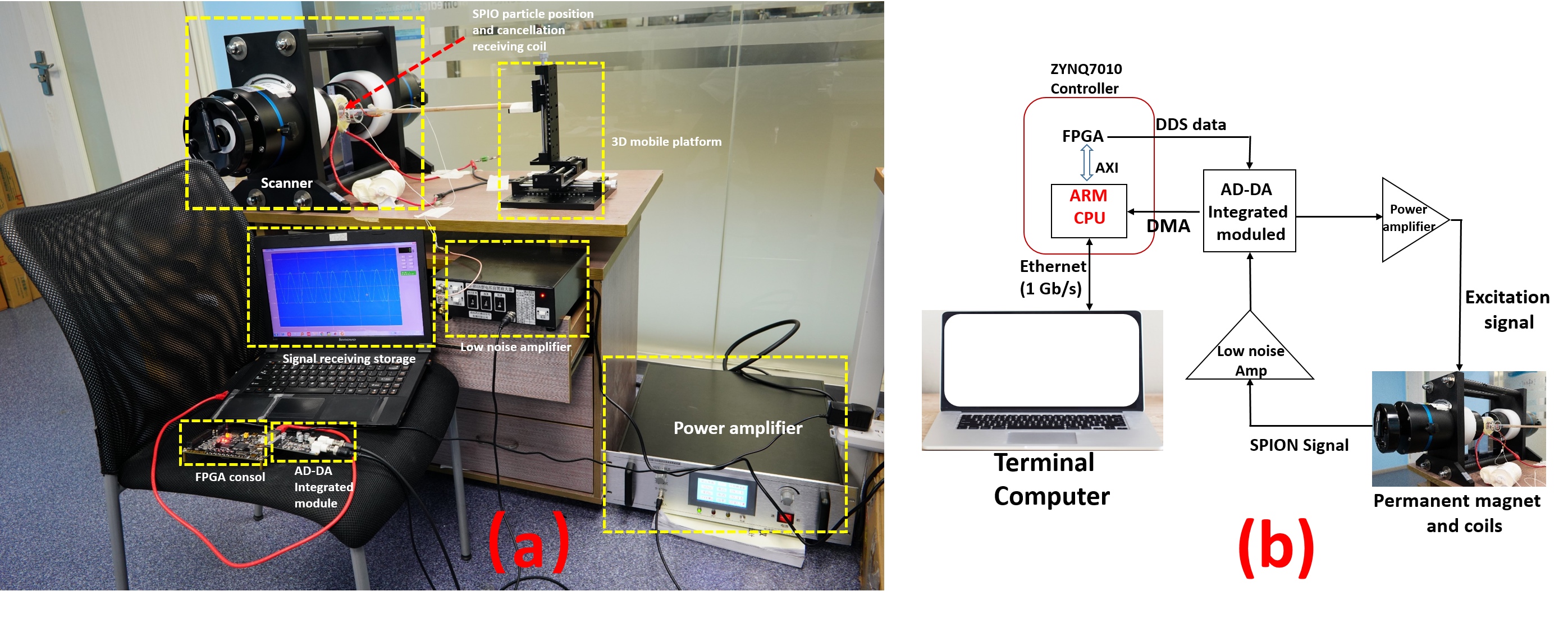
Figure 1. MPI overall system configuration, where (a) represents the overall physical connection and (b) represents the signal flow diagram. The excitation signal output from the FPGA was amplified by the power amplifier and
sent to the drive coil. The SPION signal was captured
by the ADC after passing through the low noise amplifier, which was then transmitted
to the terminal for storage and digital filtering via the 1 Gb / s UDP protocol
packet.
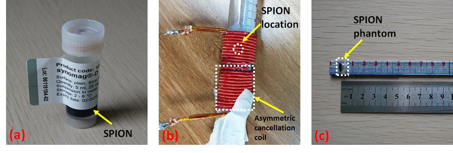
Figure 2. Experimental materials. (a) Superparamagnetic iron-oxide
nanoparticles (SPIONs) with a particle size of 50 nm and a
concentration of 25 mg/ml were used in the experiments.
(b) The overall view of the receiving coil, where the white dotted line indicates the location of the
particle and the cancellation coil. (c) The phantom that was moved during the experiment.
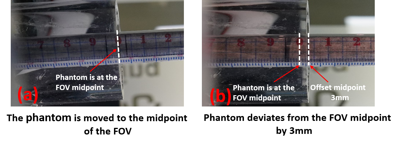
Figure 3. The process of phantom
moved inside the FOV, where (a) indicates that the phantom was at the FOV midpoint, as a reference
point for the rear movement, and (b) shows that the phantom
moved reference point was 3 mm inside the FOV.
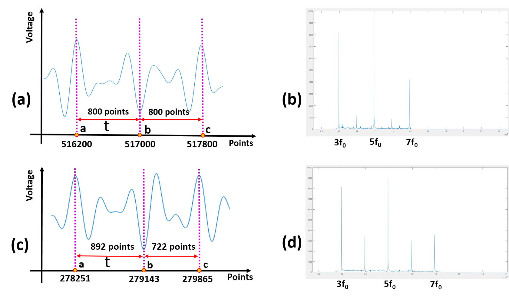
Figure 4. A time-domain map after the digital bandpass filter filtered out the fundamental and noise of FFP traversing the FOV for one cycle was demonstrated by (a) and (c), respectively, when the phantom was moved to the FOV midpoint and the offset midpoint of 3 mm. The spectrograms of (a) and (c) were illustrated through (b) and (d), respectively.
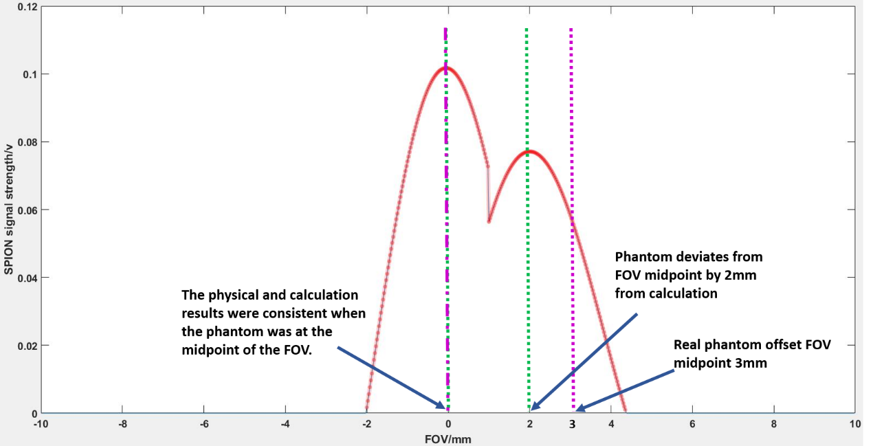
Figure 5. The signal time domain maps of (a) and (c) in Figure 4 were optimized and combined to map to the FOV distance. The calculation results of Eq. (1) and (2) have shown when the actual phantom was at the midpoint of the FOV, the calculated position was consistent with the actual position. However, when the actual phantom offsets the FOV midpoint by 3 mm, the calculated distance and the actual distance were 1 mm error. Here, they were shown by the green and purple dashed lines, respectively.