1244
Estimation of stable whole-brain effective-connectivity characterization of mental disorders1Brigham and Women's Hospital, Boston, MA, United States, 2Harvard Medical School, Boston, MA, United States
Synopsis
We propose an algorithm to estimate whole-brain effective connectivity measures by integrating structural connectivity matrix between brain regions and resting-state functional MRI data. Our algorithm first uses the Lyapunov inequality from control theory to ensure that the estimated whole-brain dynamic system is stable and physically meaningful. Then, the effective connectivity measure is characterized by a novel conditional causality measure. We applied the proposed algorithm to a public dataset which consisted of healthy controls (n=94), patients with schizophrenia (n=45), bipolar (n=44) and ADHD (n=37). Our results show that the proposed approach provides reliable estimation brain-network features of these brain disorders.
Introduction
Functional connectivity (FC) is a standard approach to measure the functional synchronization between brain regions. Although it is sensitive to brain abnormalities[1-3], it does not provide information about the direction of the connectivity[5]. On the other hand, effective connectivity is a more powerful approach to estimate the direction of information flow within brain networks. Dynamic causal modeling and Granger causality analysis[4-7] are standard approaches for analyzing effective connectivity of brain networks. These approaches use either linear or bilinear models to characterize functional brain dynamics. Although these methods have been used to investigate mental disorders, most applications either focus on small-scale networks or pairwise connections. Although several heuristics have been proposed to ensure the stability of brain network dynamics, these algorithms are not efficient for larger scale whole-brain network analysis. In this work, we propose a novel estimation algorithm based on the Lyapunov inequality from control theory[8] to identify a stable whole-brain dynamical system with structural constraints. We demonstrate an application of this approach to characterize brain network features of several mental disorders using a public dataset.Method
Structural connectivity estimation: The dataset was obtained from the UCLA consortium for neuropsychiatric phenomics LA5c study[9]. The data consisted of 94 controls, 45 patients with schizophrenia, 44 patients with bipolar and 37 patients with ADHD. We first used our multi-fiber tractography algorithm[10] to compute whole-brain tractography. Then we used the WMQL toolbox[12] and the Freesurfer[11] label maps to compute the whole-brain structural connectivity matrix between 93 cortical and subcortical regions from the whole brain. To reduce the possibility of false positives, we used only those connections that were consistently traced in all subjects.Stable whole-brain dynamical system estimation with structural constraints: Resting state functional MRI data consisted of 152 volumes with TR=2s, matrix size = 64x64x34, slice thickness = 4mm. The datasets were processed using the standard pipeline based on SPM[13]. The average time-series signal from each of the 93 brain regions was extracted. For effective connectivity analysis, we used a vectorial autoregressive model to characterize the temporal dependence of the time-series data. To ensure the stability of the estimated model, we restricted the system matrix A to satisfy that $$$P-APA^T\geq0$$$ where P is a positive definite sample covariance matrix of the measured data. The stability of A is guaranteed by the Lypunov stability criteria[8]. Furthermore, we set the entries of A that correspond to indirect structural connections to zero. Model parameters were estimated by solving a convex optimization problem using the cvx toolbox[14].
Conditional frequency-domain causality measure: Based on the estimated model parameters, we computed the conditional frequency-domain causality measure proposed in our previous work[7]. The conditional Granger causality measure is able to quantify the intrinsic information flow between two interconnected brain regions by regressing out the influence from other regions. We used the average value of frequency-domain causality measure in the 0 – 0.1 Hz interval as the effective connectivity measure.
Normalization with respect to controls: The brain networks of patients with mental disorder consist of disease-related connections as well as normal connections similar to controls. To increase the sensitivity of effective connectivity to brain abnormalities, we normalized the estimated brain connectivity with respect to the corresponding measure of healthy controls using the z-score. In this way, the effective connectivity measure of healthy connections is reduced. We further applied principle component analysis (PCA) to estimate the dominant network components from the three groups of patients and analyze the difference between the four groups using the network scores.
Results
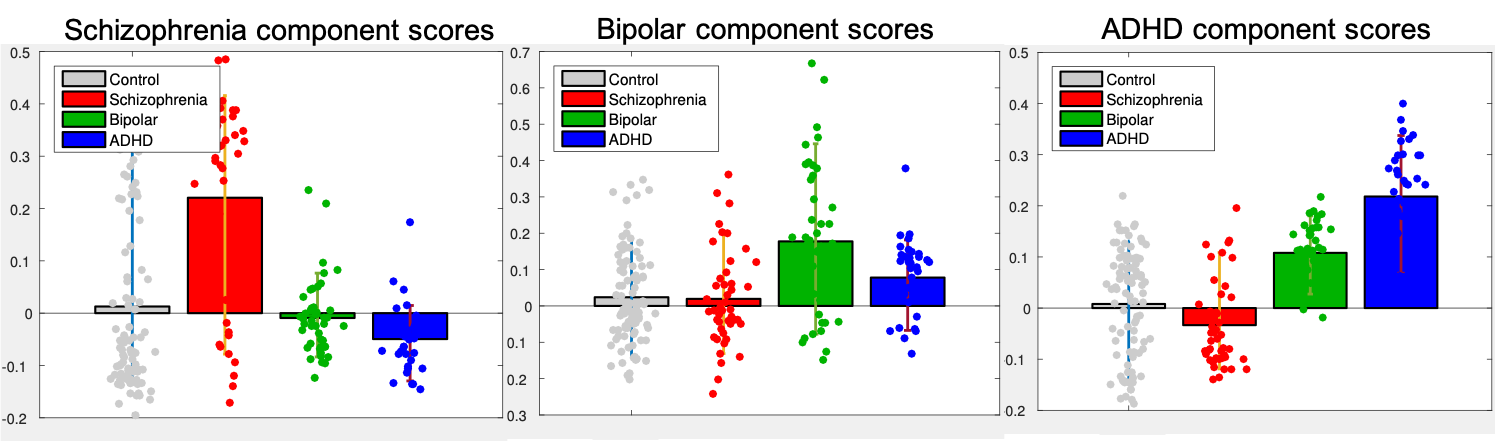
A stable linear dynamic system has all it eigenvalues within the unit disk on the complex plane. Figures (1) shows the scatter plot of eigenvalues of the estimated system matrices of all subjects. Clearly, all eigenvalues are within the unit circle indicating all systems are stable.Figure (2) shows the scatter plot of the three principle component scores where the three groups of patients are shown by different colors. It can be seen that most patients with schizophrenia (red) are clearly separated from other subjects. The few outliers may be of different biotypes. In more detail, Figure (3) shows each one-dimensional principle component score of four groups of subject. In particular, the schizophrenia component scores of patients with schizophrenia are significantly different from the schizophrenia component scores of other subjects (p<0.01). Similarly, the bipolar (or ADHD) component scores of patients with bipolar (or ADHD) are also significantly different from the corresponding scores of other groups (p<0.01).
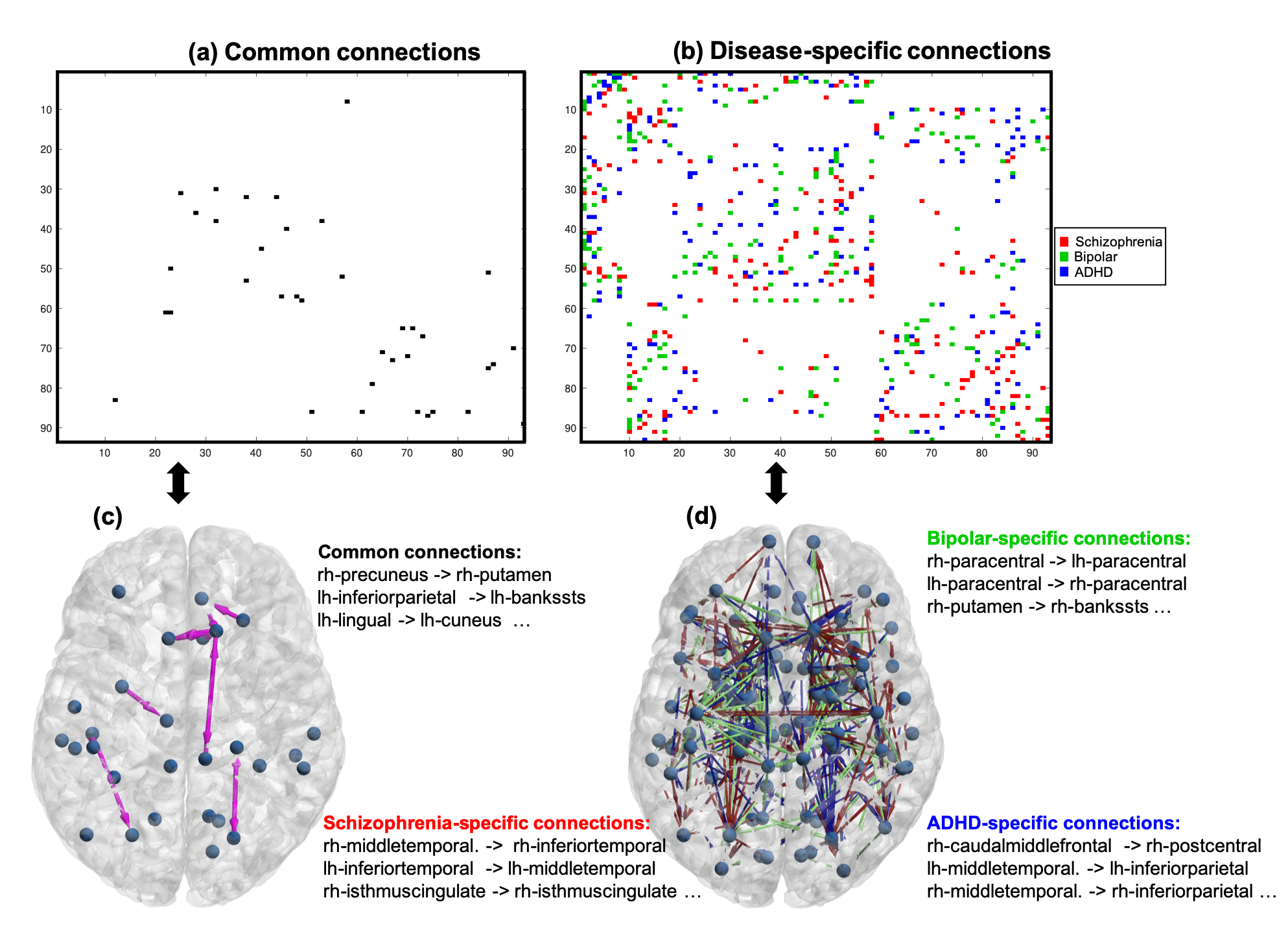
Figures (4a, 4c) show the common effective connections among the three components. Figures (4b, 4d) illustrate disease-specific effective connections, where the red, green and blue colors indicate the connections that only exists in schizophrenia, bipolar and ADHD related components. The brain regions related to some common and disease-specific connections are also listed in the figure.
Discussion and Conclusions
We introduced an algorithm for estimating stable whole-brain effective connectivity based on optimization and control theory. We illustrated an application of this approach to identify disease-specific brain network features. The relation between the estimated network components and clinical outcomes will be explored in future work.Acknowledgements
This work is supported in part by NIH grants R21MH116352, R21MH115280, K01MH117346, R01MH116173, R01MH111917, R01MH074794, P41EB015902.References
[1] M-E.
Lynall, D.S. Bassett, R. Kerwin, P. J. McKenna, M.
Kitzbichler, U. Muller, and Ed Bullmore, “Functional Connectivity and Brain Networks in Schizophrenia”, The Journal of Neuroscience, (2010);
30(28):9477–9487.
[2]
M.L. Phillips, E. Vieta, “Identifying functional neuroimaging biomarkers of
bipolar disorder: toward DSM-V”, Schizophr Bull, (2007); 33:893-904.
[3]
Y. Paloyelis, M.A. Mehta, J. Kuntsi and P. Asherson, “Functional MRI in ADHD: a
systematic literature review”, Expert Review of Neurotherapeutics, (2007) 10:
1337-1356.
[4] K.
J. Friston, L. Harrison, and W. Penny, “Dynamic causal modelling”, Neuroimage,
(2003); 19, 1273–1302.
[5]
K. J. Friston, “Functional and effective connectivity: a review”, Brain
Connect, (2011); 1(1):13-36.
[6]
K. J. Friston, R. Moran, and A. K. Seth, “Analysing connectivity with Granger
causality and dynamic causal modelling”, Curr. Opin. Neurobiol (2013); 23:172–178.
[7]
L. Ning and Y. Rathi, “A Dynamic Regression Approach for
Frequency-Domain Partial Coherence and Causality Analysis of Functional Brain
Networks”, IEEE Trans Med Imaging (2018); 37(9): 1957-1969.
[8] P.C. Parks, "A. M.
Lyapunov's stability theory—100 years on". IMA Journal of Mathematical
Control & Information, (1992). 9 (4): 275–303.
[9]
R. Poldrack, E. Congdon, W. Triplett, et al. A phenome-wide examination of neural and cognitive function”. Sci
Data 3, 160110 (2016).
[10] J.G.
Malcolm, M.E.
Shenton, Y.
Rathi. “Filtered multitensor tractography”.
IEEE Trans Med Imaging. (2010);29(9):1664-75.
[11] B.
Fischl, FreeSurfer. Neuroimage. (2012), 15;62(2):774-81.
[12]
D. Wassermann, N. Makris, Y. Rathi, M. Shenton, R. Kikinis, M. Kubicki, Westin
CF. On describing human white matter anatomy: the white matter query language.
Med Image Comput Comput Assist Interv. 2013;16(Pt 1):647-54.
[13] K.J. Friston, J. Ashburner, S.J. Kiebel, T.E.
Nichols, and W.D. Penny, editors. Statistical
Parametric Mapping: The Analysis of Functional Brain Images. Academic Press, 2007.
[14] M.
Grant, S. Boyd. CVX: Matlab software for disciplined convex programming, version
2.0 beta. http://cvxr.com/cvx, September 2013.
Figures
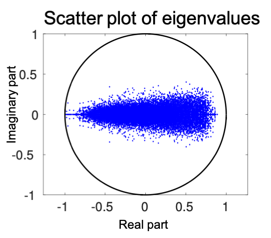
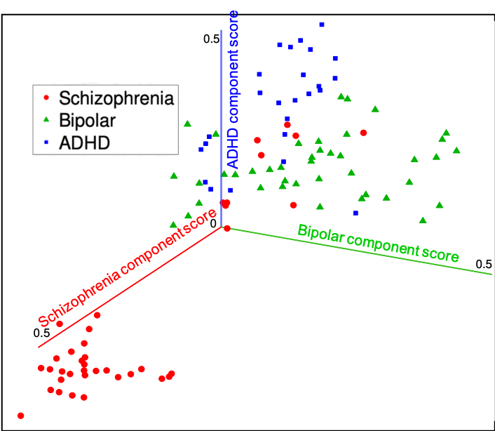
Figure 2: Scatter plot of the three disease-specific component scores of patients with schizophrenia (red), bipolar (green) and ADHD (blue). Most schizophrenia patients have significantly higher schizophrenia component scores than the other two groups. The few outliers of schizophrenia patients may be of different biotypes. Bipolar and ADHD patients are also separated by the corresponding component scores.