1172
Spinal Cord Segmentation and T2*-relaxation times of GM and WM within the Spinal Cord at 9.4T1High-field Magnetic Resonance, Max-Planck-Institut for biolog. Cybernetics, Tübingen, Germany, 2Institute for Biomedical Magnetic Resonance, University Hospital Tübingen, Tübingen, Germany, 3Advanced Imaging Research Center, University of Texas Southwestern Medical Center, Dallas, TX, United States
Synopsis
This study presents the first investigations with algorithmic spinal cord-segmentation, as well as gray matter/white matter-segmentation within the spinal cord, at the ultrahigh field strength of 9.4T. On multi-echo gradient-echo acquisitions from three subjects, the tested algorithms perform the segmentations correctly. Based on these multi-echo data, pixel-wise T2*-relaxation time maps were calculated. By means of the segmentations, averaged T2*-times of 24.88ms +- 6.68ms for gray matter and 19.37ms +- 8.66ms for white matter, were calculated.
Introduction
Nowadays, for clinical diagnostic and research investigations of the human spinal cord (SC), magnetic-resonance-imaging (MRI) is an indispensable method. Tissue changes in gray matter (GM) and white matter (WM) within the SC have been associated to several neurological disorders such as SC injury, neoplastic lesions1, or multiple sclerosis2. Based on 3T MRI-acquisitions, the segmentation of the entire SC is routinely done to measure SC atrophy3 or to support surgical planning4. Recently, SC-detection and GM-segmentation of 7T human SC images were performed manually5 as well as automatically6 using the segmentation algorithms of the spinal cord toolbox7.This work presents the first investigations of algorithmic SC-detection, as well as GM/WM- segmentation of high-resolution human SC images acquired at 9.4T. Furthermore, as tissue relaxation rates change with increasing B0 field strength8, T2*-relaxation time maps are calculated and T2*-times of GM and WM in the human SC at 9.4T are presented.
Methods
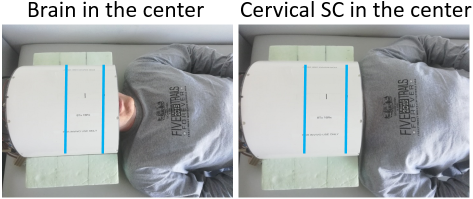
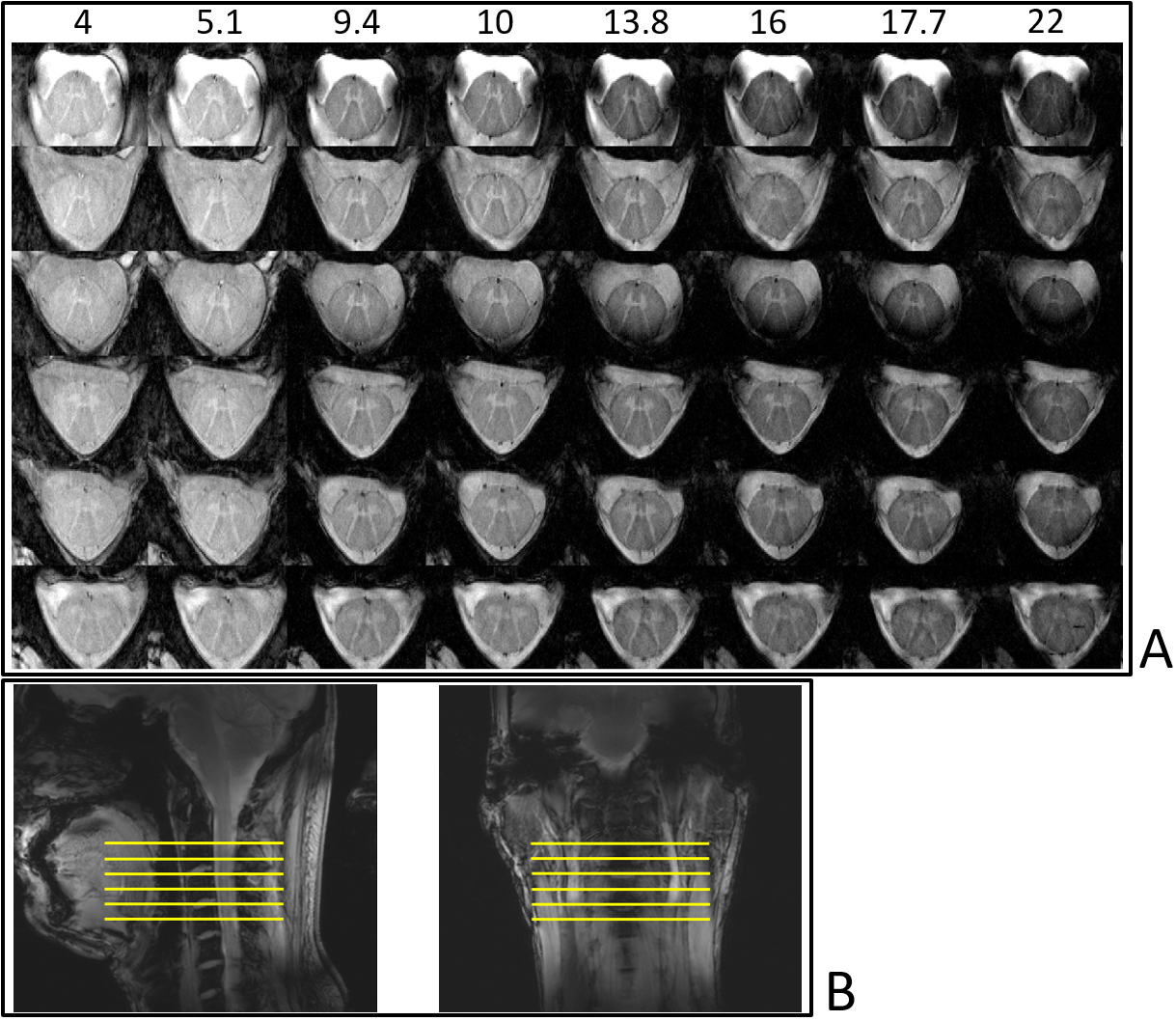
All experiments were performed on a Siemens (Erlangen, Germany) Magnetom 9.4T whole-body MRI scanner. Analog to Geldschläger et al.9, for RF-transmission and reception, a 16-channel tight-fit array10, consisting of eight transceiver surface loops and eight receive-only vertical loops, was used. The coil was originally constructed for human brain scans with emphasis to enhance the Signal-to-Noise-Ratio (SNR) in deep structures, but through subject replacing (Figure 1) it can be used to image the cervical SC, as well.9.4T anatomical imaging data was acquired using an axial T2*-weighted multi-echo gradient-echo (GRE)-sequence (field of view: 140x140mm2, In-plane res.: 0.23x0.23mm2, Number of slices: 12, slice thickness: 3mm, Repetition time (TR): 500ms, FA: 50°, 4 echoes, Acquisition time: 5min:04sec, 2D). On three different healthy volunteers, the sequence was applied twice, respectively: once with the echo times (TEs) 4, 10, 16 and 22ms and once with the TEs 5.1, 9.4, 13.8 and 17.7ms (analog to the TEs from Massire et al.6).
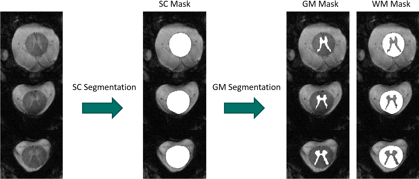
The T2*-weighted anatomical imaging data acquired at a TE of 9.4ms were segmented with the Spinal-Cord-Toolbox (SCT)7 (PropSeq-algorithm11 for SC-segmentation and deep-learning-algorithm12 for GM-segmentation).
Pixel-wise T2*-time calculation was performed with a mono-exponential fit, based on the eight sample points per pixel acquired with the multi-echo GRE-sequence. The fitting was performed with a nonlinear least-squares algorithm using Matlab (The Mathworks, Natick ,MA, USA).
Using the beforehand obtained GM/WM-masks, the T2*-time of GM and WM were averaged.
Results
In Figure 2, the anatomical imaging results from one subject, are depicted. It is visible, that with increasing TE, the signal decays. For a TE between 9.4 ms and 13.8 ms a good GM/WM contrast is achieved and a TE of 9.4 ms is the best compromise between SNR and contrast. At longer TEs, signal-dropouts can be seen in slices located next to intervertebral disks.Represented on the example of three slices acquired from another subject, Figure 3 shows the segmentation results. Both, the SC-segmentation and the GM-segmentation algorithm delivers the correct masks. For the three scanned volunteers, the segmentation algorithms produced correct results for all acquired slices when using images acquired with a TE of 9.4ms.
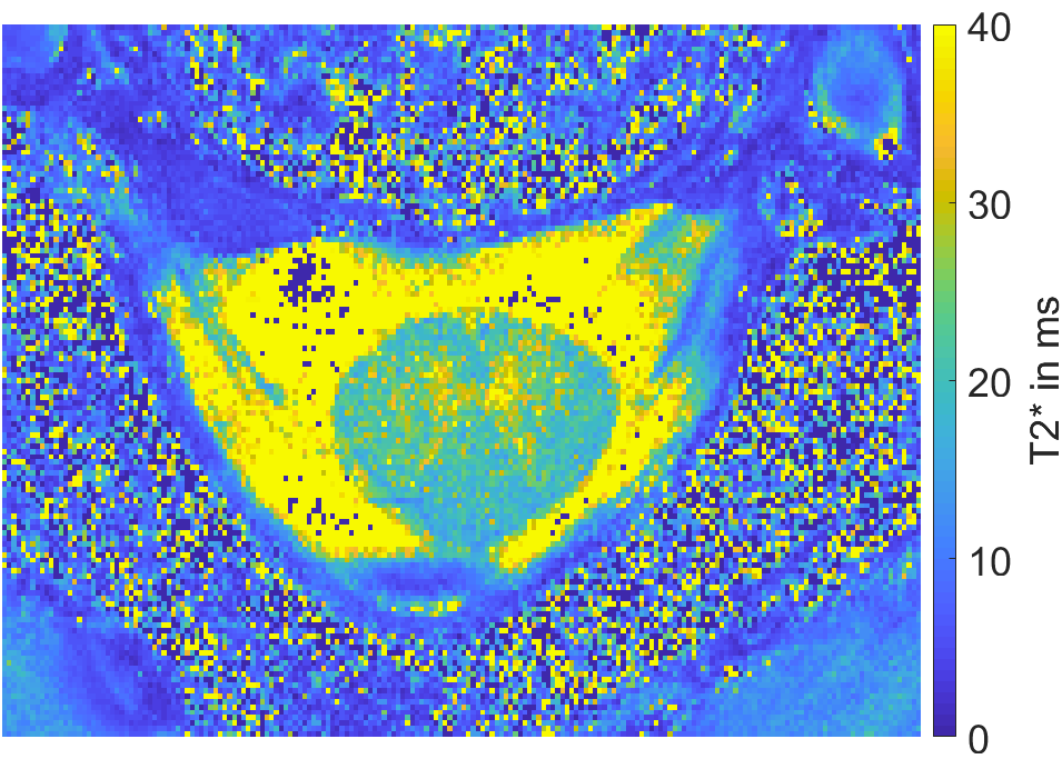
Figure 4 shows an example slice of a T2*-map. The SC is recognizable and the GM and WM within the SC is distinguishable. T2*-slices in which these tissue types were not recognizable at all, were excluded from the averaging. For the cervical SC at 9.4T the calculated mean T2*-time for GM is 24.88ms +- 6.68ms and for WM 19.37ms +- 8.66ms.
Discussion
It was shown, that algorithmic SC-segmentation and GM/WM-segmentation is possible using high-resolution T2*-weighted images acquired at 9.4T with the proposed brain coil. The employed algorithms from the SCT7 produced correct SC and GM/WM masks for all tested datasets. That leads to the assumption that the algorithms work reliably for 9.4T human SC images and have a low probability to produce wrong segmentations in general.The presented averaged T2*-times in the human SC at 9.4T are consistent with the literature, although an uncertainty remains when using this pixel-by-pixel fit method (see noise in Figure 4 and the resulting relatively high standard deviation). Additionally, the subject database size was relatively small (3 subjects). As expected, the T2*-times from the cervical SC at 7T (GM: 29.3ms +- 4.5ms, WM: 23.5ms +-5.7ms)6 are slightly higher, while the T2*-times at 9.4T for the human brain (GM: 23.8ms +- 1.0ms, WM: 19.2ms +- 0.9ms)13, are very similar to the values calculated for the SC at 9.4T.
Through the application of other sequences (for example MP2RAGE14 or T2W) in the future, T1- and T2-relaxation time measurements need to be performed, in order to complete the set of tissue relaxation times for the SC at 9.4T.
Conclusion
With this work the next step into SC research at a B0 field strength higher than 7T was done. With a coil, originally optimized for maximal SNR in deep brain structures, we were able to acquire high-resolution anatomical SC data on which algorithmic SC-segmentation, as well as GM/WM-segmentation, reliably works. The T2*-times of GM and WM in the human SC at 9.4T were presented. This might open new possibilities in the field of SC-research and clinical patient care at ultra-high-field. Knowing the T2*-relaxation time allows optimization of imaging parameters and potentially enables improvements in sensitivity and contrast.Acknowledgements
Funding by the European Union (ERC Starting Grant, SYNAPLAST MR, Grant Number: 679927) is gratefully acknowledged.References
1. Amukotuwa SA, Cook MJ. SPINAL DISEASE: NEOPLASTIC, DEGENERATIVE, AND INFECTIVE SPINAL CORD DISEASES AND SPINAL CORD COMPRESSION. In Neurology and Clinical Neuroscience.: Elsevier; 1999. p. 511-538.
2. Schlaeger R, Papinutto N, Panara V, Bevan C, Lobach IV, Bucci M, et al. Spinal cord gray matter atrophy correlates with multiple sclerosis disability. Annals of Neurology. 2014 Aug; 76: 568-580.
3. Lin X, Tench CR, Evangelou N, Jaspan T, Constantinescu CS. Measurement of Spinal Cord Atrophy in Multiple Sclerosis. Journal of Neuroimaging. 2004 Jul; 14: 20-26.
4. Mukherjee DP, Cheng I, Ray N, Mushahwar V, Lebel M, Basu A. Automatic Segmentation of Spinal Cord MRI Using Symmetric Boundary Tracing. IEEE Transactions on Information Technology in Biomedicine. 2010 Sep; 14: 1275-1278
5. Sigmund EE, Suero GA, Hu C, McGorty K, Sodickson DK, Wiggins GC, et al. High-resolution human cervical spinal cord imaging at 70.167emT. NMR in Biomedicine. 2011 Dec; 25: 891-899.
6. Massire A, Taso M, Besson P, Guye M, Ranjeva JP, Callot V. High-resolution multi-parametric quantitative magnetic resonance imaging of the human cervical spinal cord at 7T. NeuroImage. 2016 Dec; 143: 58-69.
7. Leener BD, Lévy S, Dupont SM, Fonov VS, Stikov N, Collins DL, et al. SCT: Spinal Cord Toolbox, an open-source software for processing spinal cord MRI data. NeuroImage. 2017 Jan; 145: 24-43.
8. Chavhan GB, Babyn PS, Thomas B, Shroff MM, Haacke EM. Principles, Techniques, and Applications of T2∗-based MR Imaging and Its Special Applications. RadioGraphics. 2009 Sep; 29: 1433-1449.
9. Geldschläger O, Manohar SM, Wright A, Avdievitch N, Henning A. First MRI of the human spinal cord at 9.4T. In 27th ISMRM; 2019; Montreal, Canada.
10. Avdievich NI, Giapitzakis IA, Pfrommer A, Borbath T, Henning A. Combination of surface and `vertical' loop elements improves receive performance of a human head transceiver array at 9.4 T. NMR in Biomedicine. 2017 Dec; 31: e3878.
11. Leener BD, Kadoury S, Cohen-Adad J. Robust, accurate and fast automatic segmentation of the spinal cord. NeuroImage. 2014 Sep; 98: 528-536.
12. Perone CS, Calabrese E, Cohen-Adad J. Spinal cord gray matter segmentation using deep dilated convolutions. Scientific Reports. 2018 Apr; 8.
13. Pohmann R, Speck O, Scheffler K. Signal-to-noise ratio and MR tissue parameters in human brain imaging at 3, 7, and 9.4 tesla using current receive coil arrays. Magnetic Resonance in Medicine. 2015 Mar; 75: 801-809.
14. Marques JP, Kober T, Krueger G, Zwaag W, Moortele PFV, Gruetter R. MP2RAGE, a self bias-field corrected sequence for improved segmentation and T1-mapping at high field. NeuroImage. 2010 Jan; 49: 1271-1281.
Figures