Introduction

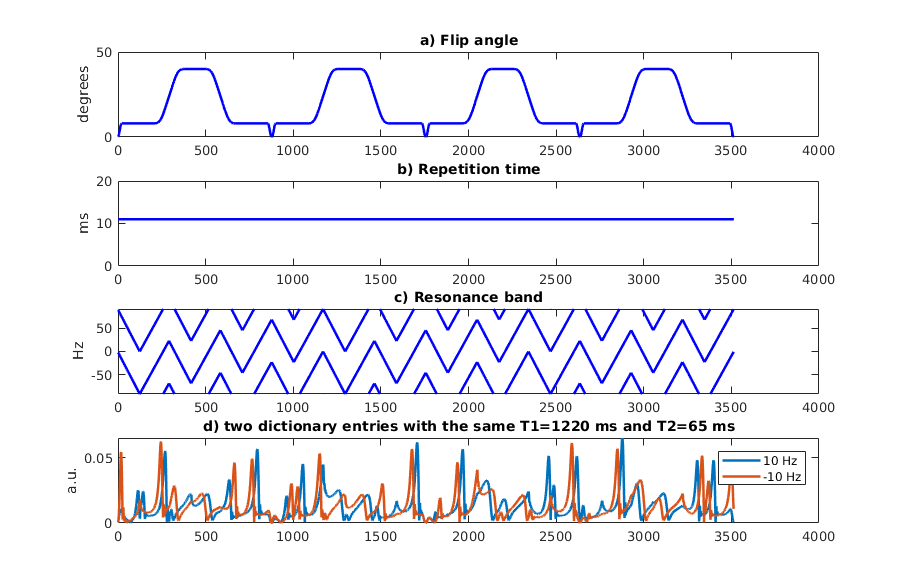
Magnetic Resonance Fingerprinting¹ (MRF) is a quantitative imaging technique for simultaneous mapping of multiple tissue properties and system parameters. Recently, MRF was extended to map T2* and off-resonance (Δf) alongside T1 and T2². MRF with quadratic RF pulses (MRFqRF) sweeps the on-resonance frequency linearly between -1/(2*TR) to 1/(2*TR) in time by modulating the RF phase with a quadratic function (Figure 1). Dynamic sweeping of off-resonance frequencies makes the signal evolutions different for all the time points and stable against random noise (Figure 2). In this work, stability of MRFqRF for off-resonance mapping was explored for use in temperature monitoring of aqueous tissues. However, the conventional temporal resolution of MRFqRF is much slower than what is required for temperature monitoring of thermal therapies (40s vs 3s). Here, we performed proof of concept experiments with the MRFqRF framework to optimize it for fast and continuous mapping of Δf for temperature quantification.

Methods

Experimental setup
A tofu phantom was immersed in a water bath and placed at isocenter of a 3T MRI scanner (Skyra, Siemens). The laser ablation device’s applicator (LaserPro 980, PhotoMedex) and a fiber optic temperature probe (Luxtron, LumaSense Technologies) were placed together in the center of the phantom. A second temperature probe was positioned inside the phantom away from the site of the heating for reference measurements. For each experiment, the tofu was heated with the laser ablator for ~20 s at 1.5 W of Continuous Wave power, followed by subsequent cooling (total of 6:40 minutes per experiment).
Data acquisition
To approach the temporal resolution of conventional proton resonant frequency-shift thermometry (~3s), the number of time points per one MRFqRF scan was reduced. This was achieved by sweeping the off-resonance frequency faster with respect to MRFqRF with 3516 time points (0.72 Hz/TR) by adjusting the quadratic RF function (2x in 1752 time points with 1.44 Hz/TR and 4x in 876 time points with 2.88 Hz/TR). The original flip angle pattern was resampled, and the same four block structure was preserved for consistency. The phantom setup described above was scanned for the 6:40 minutes with three different 2D MRFqRF versions during heating and cooling of the phantom.
Reconstruction and post-processing
2D MRFqRF data were reconstructed after compression with randomized SVD³. The compressed data were matched to a compressed dictionary, which was also partially undersampled in the tissue dimension. The low resolution in the tissue dimension was recovered with quadratic interpolation⁴ after the matching. The relatively strong gradients needed for MRFqRF acquisition can cause eddy currents and frequency drifts over time (~4 Hz/min), which need to be removed to see underlying off-resonance changes due to temperature. For automated estimation of frequency drift, Independent Component Analysis (ICA)⁵ was run on the dynamic Δf series of an 11x11 ROI from a region where no temperature change is expected. The component that describes the linear frequency drift was then removed from all voxels in the dynamic Δf series. Finally, the reconstructed off-resonance maps were converted to ΔT with the following equation⁶, where $$$γ$$$ is the gyromagnetic ratio in MHz/T, B₀ is the field strength in Tesla, and n is the dynamic scan number. $$ \triangle T_n=\frac{\triangle f_n - \triangle f_0}{-0.01*\gamma*B_0} $$

Results

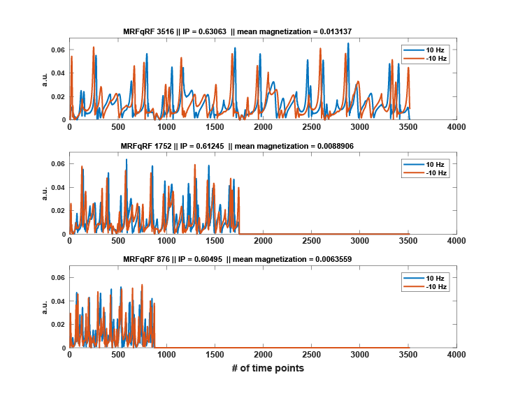
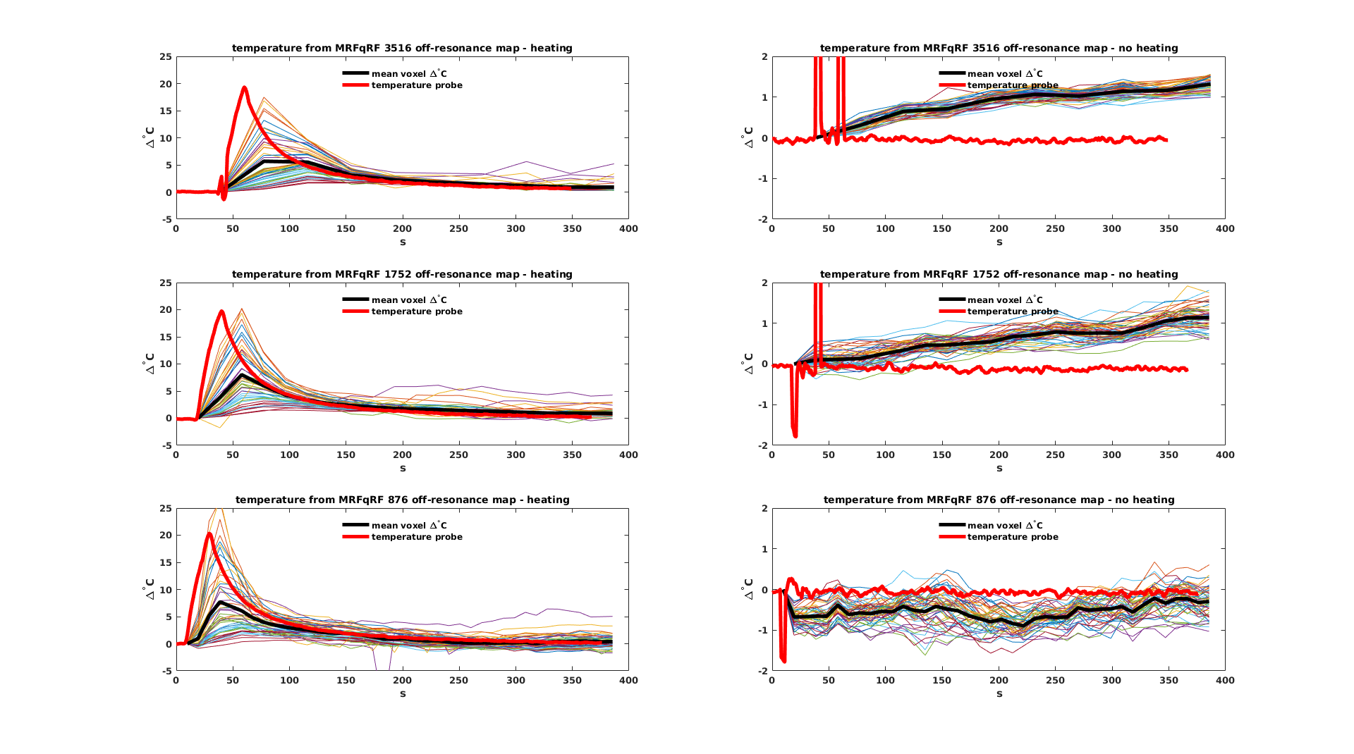
Figure 3 compares the signal evolutions of two different dictionary entries with matching T1 and T2 for MRFqRF 3516/1752/876. Inner product of signal evolutions is similar across number of time points, but SNR is reduced as the number of time points decrease. The ΔT of the laser ablation experiment computed from MRFqRF Δf maps using 3516/1752/876 time points is plotted in Figure 4. All three acquisitions were able to detect heating. Reducing the number of time points brings finer resolution sampling of the heating curve through time, but also increased noise, which can be inferred from the standard deviation over voxels around the not heated point.

Discussion

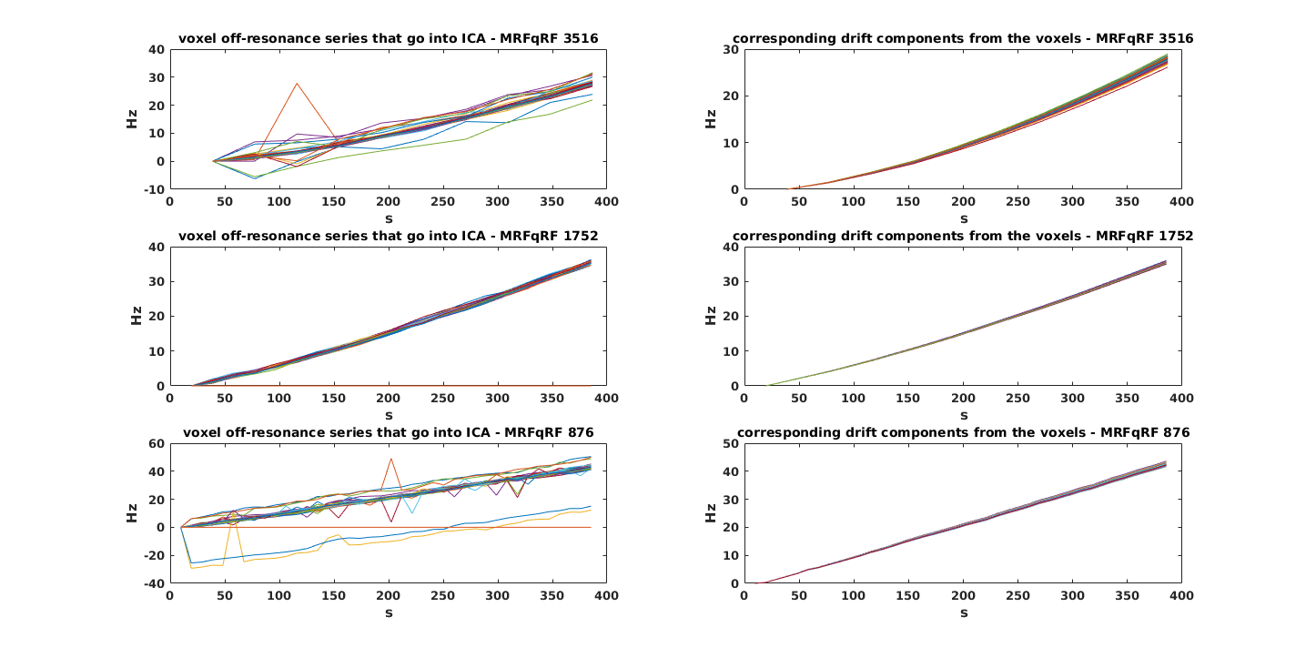
While heating occurred relatively quickly (~1 °C/s), cooling was much slower, allowing even the slowest MRFqRF version (40s per scan) to capture the general trend of temperature. Relatively stable MRFqRF 876 can sample the heating curve 4x faster, but it is also significantly slower than clinical need. The SNR with faster MRFqRF translates into slightly noisier ΔT estimations, but the relatively stable inner product is still the dominant factor. This observation might be useful for future optimization. Frequency drift correction is extremely important to be able to focus on small off-resonance fluctuations triggered by changes in temperature. Simple summation of voxel time series or fitting a linear function might be suboptimal considering the large fluctuations that are possible (Figure 5, left). ICA is able to detect the frequency drift component consistently (Figure 5, right).

Conclusions

This work demonstrates the first steps for temperature monitoring with an MRF framework. However, clinically-feasible ablations would benefit from further increases in temporal resolution with faster sampling of the heating curve. Additionally, no information can be obtained about heating in adipose tissue with this current implementation due to the use of off-resonance changes for temperature computation. Improvements to acquisition speed and contrast in multiple tissue types is necessary, before it can be used in real-time treatment monitoring and is the subject of future work⁷.

Acknowledgements

The work was supported by Siemens Healthcare and a cooperative grant between the University of Colorado and NIST. Authors would like to thank Will Grissom for use of the temperature probes.