1122

Validation of RF induced temperature increase in phantom and in living human tissue: a comparison study

Shubham Gupta¹, Keiji Tanaka¹, and R. Allen Waggoner¹
¹Laboratory for Cognitive Brain Mapping, RIKEN Center for Brain Science, Wakoshi, Saitama, Japan

Synopsis

In this study, we compared the temperature increase in a phantom and three human legs that were calculated by the simulations, measured by the MR-thermometry, and the optical thermocouples (phantom only), with good agreement between the modalities. IEC guidelines require simulations of SAR along with validation in phantoms to ensure safety. While it is likely impossible to simulate every possible pulse shape and phase combination in a pTx system with a large number of transmit channels, the results we present here suggest that simulations plus MR-thermometry could provide the verification currently lacking in pTx studies.

Introduction

MR imaging, although non-invasive, can cause burns due to radio-frequency heating. To prevent thermal injuries, the IEC¹ specifies limits for local and core temperature increase (ΔT) and specific absorption rate (SAR). While the whole-body SAR or regional SAR can be easily calculated during imaging², the estimation of local SAR depends on precise numerical simulations. During parallel transmission (pTx) MRI, each channel transmits a unique RF waveform, tailoring the combined transmit field to correct for magnetic inhomogeneities. However, this flexibility also provides the potential to inadvertently concentrate the associated electric field, thus posing a safety risk³.

Tissue temperature change is a more relevant measure of the subject-safety than SAR, and it has been shown that the SAR distributions may not always correlate well with tissue heating patterns⁴. Here we are proposing to perform MR-thermometry^2,5–8 between pTx imaging (e.g., fMRI or DTI) runs to determine if local heating has exceeded safety limits. This protocol would add a layer of safety during pTx MRI, on top of simulations. To test the validity and effectiveness of the protocol, in this study, we have compared the ΔT calculated by numerical simulations, measured by MR-thermometry, and optical thermocouples in an agar gel phantom, and that from numerical simulations and MR-thermometry in living human tissue.

Methods

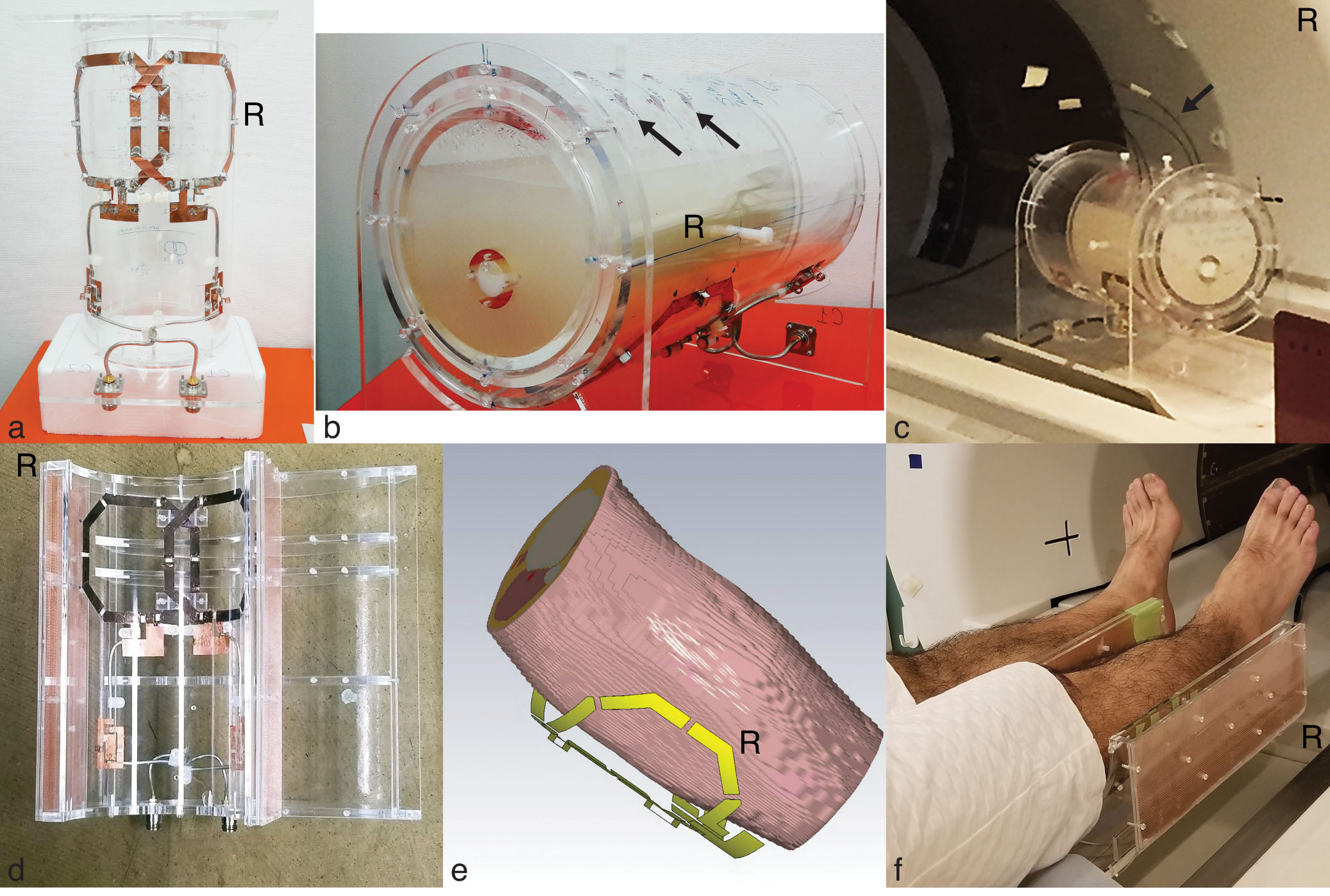
An inhouse built two-channel parallel transceive surface array coil (Figure-1a and 1d) was used to heat and image an agar phantom (figure) (15g/L agar, 4.0g/L NaCl, 0.02g/L MnCl₂) and calves of the right legs of three subjects. Heating and scanning were performed intermittently using the same coil on a 4T Agilent scanner. Four optical thermocouples were inserted at different locations to measure the ΔT (Figure-1c) in the phantom during four experiments (with different amplitude and phase combinations). The results from the three modalities, i.e., thermocouples, MR-Thermometry, and simulations, were compared. For human legs, three experiments were performed, one with each subject, and the results from two modalities, i.e., MR-Thermometry, and simulations, were compared.

An asymmetric spin-echo EPI with gradient reversal sequence^5,9,10 was used to perform Proton Resonance Frequency (PRF) shift MR-thermometry^5,11,12. The PRF shift constant was first calibrated in the phantom from the data of three separate experiments, then the result, i.e., -0.0129 ppm/°C was used for calculating the temperature maps for the phantom and the legs. For thermal simulations, the intermittent heating and scanning paradigm was modeled in the simulation software CST studio suite®. The thermocouple tips were manually mapped to the thermal simulations as point monitors. To take account of any error in mapping, in the simulations with the phantom, we also monitored 52 equidistant points in a 1-cm³ spherical region around the mapped points¹³. For the simulations with human legs, subject-specific models were developed from the anatomical images of the legs acquired on a 3T Siemens Prisma (Figure-1e).

Two separate experiments were also performed to estimate the voxelwise standard deviation (StDev) of MR-thermometry, one for the phantom and one for the human leg. Thirty-one MR-thermometry scans were performed, without heating, and the StDev of (StDev) ΔT at each voxel was calculated.

Results

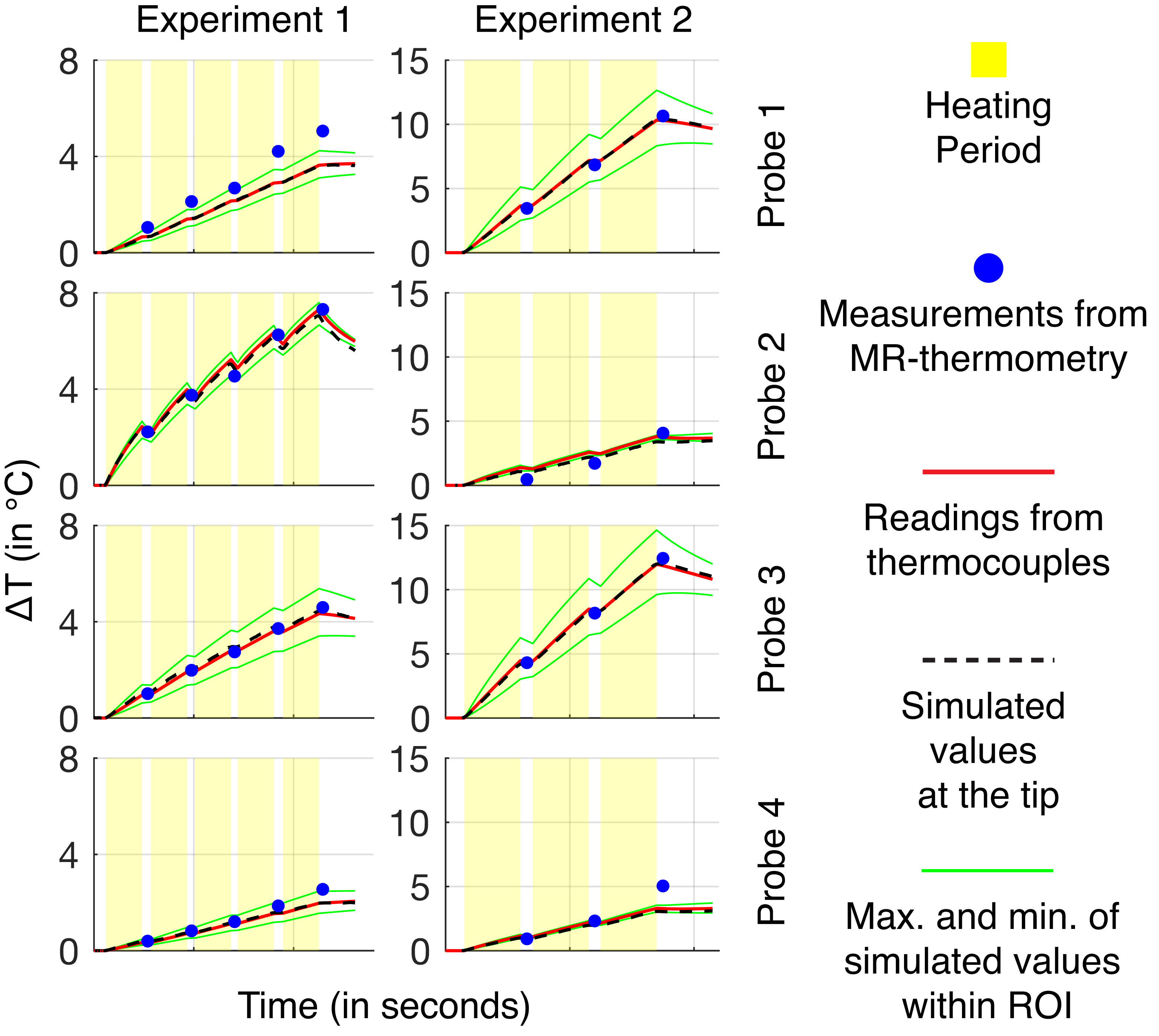
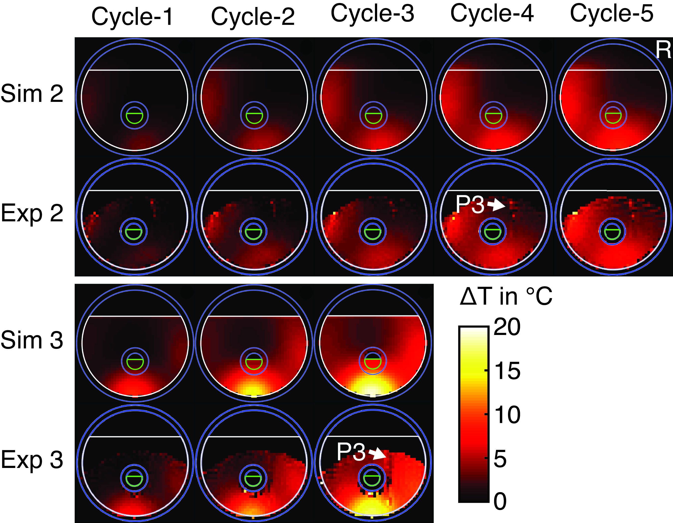
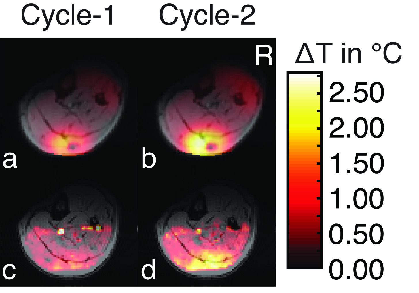
In the phantom (Figure-2 and Figure-3), the ΔT recorded from thermocouples, and calculated from the simulations were in good agreement and were between the minimum and maximum values simulated in the 1-cm³ region around the mapped thermocouple tips. The values measured by MR-thermometry were also in agreement with the other two modalities except for the cases where thermocouple locations were in the regions of low SNR¹⁴. In the region of high SNR, the differences between MR-thermometry and thermocouple values were not significantly different from zero (p-value = 0.31, unpaired t-test; average 0.055°C, 95% CI -0.053°C to 0.162°C, the maximum 0.82°C).

The experiments with human legs were performed after the approval from the “Research Ethics Committee.” The simulations were performed in advance to determine the subject’s safety during the heating experiments. The patterns from the thermal simulations and MR-thermometry results agreed (Figure-4). The peak ∆T observed at the end of the three experiments (2.6°C, 2.45°C, 2.7°C) and time-matched simulations (2.8°C, 2.3°C, 2.6°C), are also in close agreement.

The StDev of the temperature change, calculated from the StDev estimation experiment, in the region of the maximum ∆T for MR-thermometry in the phantom and human leg was 0.16°C and 0.27°C, respectively.

Discussion

This study has shown that for in-homogeneous heating in a phantom and human tissue, the compared modalities to observe ∆T are in good agreement. IEC guidelines¹ require simulations of SAR and validation in phantoms. However, in practice, pTx RF pulse parameters are determined after the subject is placed in the magnet, making phantom validation of the actual pulse parameters nearly impossible. Even with the level of sensitivity and agreement between MR-thermometry, simulations, and direct temperature measurements obtained in this study, using MR-thermometry alone in an interleaved fashion may not be sufficient to ensure that MR measurements remain within the “normal level control mode” of the IEC Guidelines¹. However, as shown here, ensuring that temperature changes remain within the “first level control mode,” seems feasible.

Conclusion

Using MR-thermometry, in combination with simulations, has the potential for ensuring subject safety in MRI studies employing parallel transmission.

Acknowledgements

Dr. Noriyuki Kishi (MD, Ph.D.) of "Laboratory for Marmoset Neural Architecture" at RIKEN Center for Brain Science for his presence for compliance with IEC Guidelines for "First Level Mode" of operation.

The study was supported by Japan Agency for Medical Research and Development under Grant Number JP18dm0207001 and by Japan Society for the Promotion of Science KAKENHI under Grant Number JP16H06564.

References

1. IEC 60601-2-33:2010 : Medical Electrical Equipment-Part 2-33 : Particular Requirements for the Basic Safety and Essential Performance of Magnetic Resonance Equipment for Medical Diagnosis. Geneva: International Electrotechnical Commission; 2010:219.

2. Oh S, Ryu Y-C, Carluccio G, Sica CT, Collins CM. Measurement of SAR-induced temperature increase in a phantom and in vivo with comparison to numerical simulation: SAR-Induced Temperature Rise. Magn Reson Med. 2014;71(5):1923-1931.

3. Webb AG, Moortele PFV de. The technological future of 7 T MRI hardware. NMR in Biomedicine. 2016;29(9):1305-1315.

4. Wang Z, Lin JC, Mao W, Liu W, Smith MB, Collins CM. SAR and temperature: Simulations and comparison to regulatory limits for MRI. Journal of Magnetic Resonance Imaging. 2007;26(2):437-441.

5. Streicher MN, Schäfer A, Ivanov D, et al. Fast accurate MR thermometry using phase referenced asymmetric spin-echo EPI at high field. Magnetic Resonance in Medicine. 2014;71(2):524-533.

6. Simonis FFJ, Raaijmakers AJE, Lagendijk JJW, van den Berg CAT. Validating subject-specific RF and thermal simulations in the calf muscle using MR-based temperature measurements. Magnetic Resonance in Medicine. 2017;77(4):1691-1700.

7. Gupta S, Waggoner RA, Tanaka K, Cheng K. Validation of RF-induced temperature increase in a phantom: comparison of numerical simulations, MR thermometry and measurements from temperature sensors. In: Proc Intl Soc Mag Reson Med. ; 2017:2651.

8. Wu M, Mulder HT, Zur Y, et al. A phase-cycled temperature-sensitive fast spin echo sequence with conductivity bias correction for monitoring of mild RF hyperthermia with PRFS. Magn Reson Mater Phy. 2019;32(3):369-380.

9. Park HW, Kim DJ, Cho ZH. Gradient reversal technique and its applications to chemical-shift-related NMR imaging. Magn Reson Med. 1987;4(6):526-536.

10. Volk A, Tiffon B, Mispelter J, Lhoste JM. Chemical shift-specific slice selection. A new method for chemical shift imaging at high magnetic field. Journal of Magnetic Resonance (1969). 1987;71(1):168-174.

11. Ishihara Y, Calderon A, Watanabe H, et al. A precise and fast temperature mapping using water proton chemical shift. Magn Reson Med. 1995;34(6):814-823.

12. Rieke V, Butts Pauly K. MR thermometry. J Magn Reson Imaging. 2008;27(2):376-390.

13. Kogan J. A New Computationally Efficient Method for Spacing n Points on a Sphere. Rose-Hulman Undergraduate Mathematics Journal. 2018;18(2, Artice 5).

14. Ronnau J, Haimov S, Gogineni SP. The effect of signal‐to‐noise ratio on phase measurements with polarimetric radars. Remote Sensing Reviews. 1994;9(1-2):27-37.

Figures

Figure-1: (a) The two-channel parallel transceive array coil made for the study. ‘R’ indicates the right-side of the coil (i.e. Ch-1). (b) The phantom used in the experiments. Arrows indicate two of the holes for thermocouple placement. (c) Setup for phantom experiments. Arrow indicates one of the thermocouples. (d) Modified coil housing for human studies. (e) Numerical model for one of the subjects with two channel array coil (Housing and shields are hidden). (f) Setup for experiments with human subjects.

Figure-2: The temperature increase during two of the four validation experiments with the phantom. The measurements from thermocouple probes and MR-thermometry (averaged within ROI near the probes' tip) and the simulated values at the mapped points are in good agreement in most of the cases. In some instances (probes 1 and 4 in experiment 1, probe 4 in experiment 2), in which the probes were placed in the regions of low SNR, the MR-thermometry results were less precise. Effective power in Experiment 1 is 0W on Ch-1 and 6.4W on ch-2; in experiment 2 is 7.5W on Ch-1 and 6.4W on ch-2 and phase of 60°.

Figure-3: The images from the left to the right show the patterns of temperature increase at the center slice in two validation experiments (same as in Figure-2) for cycles 1 to 5 for simulation (Sim) 1 & MR-thermometry (Exp) 1 and for cycles 1 to 3 for Sim 2 & Exp 2 (15 min of heating followed by MR-thermometry). MR-thermometry images are masked to exclude regions of low SNR. The blue lines indicate the structures of the phantom shell and lard tube. The white and green lines indicate the outer contours of agar gel and lard, respectively. The white arrows with P3 indicate the positions of probe 3.

Figure-4: The patterns of temperature increase in the leg of one of the three subjects at the center slice (left to right; cycles 1 & 2 for simulation (a & b) & MR-thermometry (c & d). During each heating and scanning cycle, the leg was heated for 5 min followed by MR-thermometry (Effective power: 3.5W on Ch-1 and 3.2W on ch-2 and phase difference of 60°). MR-thermometry images are masked to exclude regions of low SNR. Simulation maps and MR-thermometry maps are overlaid on anatomical images.

Proc. Intl. Soc. Mag. Reson. Med. 28 (2020)

1122