1110

Venular Cerebral Blood Volume (vCBV) Mapping Using Fourier-Transform Based Velocity-Selective Pulse Trains

Wenbo Li^1,2, Peter van Zijl^1,2, and Qin Qin^1,2
¹Department of Radiology, Johns Hopkins University School of Medicine, Baltimore, MD, United States, ²F.M. Kirby Research Center for Functional Brain Imaging, Kennedy Krieger Institute, Baltimore, MD, United States

Synopsis

A new method is proposed to quantify the venular cerebral blood volume (vCBV) by using Fourier-transform based velocity-selective inversion (FT-VSI) to null the arterial blood signal while using Fourier-transform based velocity-selective saturation (FT-VSS) to suppress the tissue signal. Compared to previous schemes, the proposed method potentially has higher SNR and is more robust to tissue signal fluctuations attributed to system instabilities and physiological motion. The contamination of cerebrospinal fluid (CSF) signal is also corrected for by taking an extra image at a second echo with long TE. Using this method, vCBV of five volunteers were measured at 3T.

Introduction

Venular cerebral blood volume(vCBV) is an important parameter for understanding the BOLD effect. Previously, qBOLD^1,2 and a hyperoxia-based method^3,4 were designed to measure vCBV, but suffered from mutual coupling of parameters in the BOLD model and the validity of the assumption that CBF and CMRO₂ remain unchanged during a hyperoxia challenge. Others have proposed different spin labeling approaches using flow-dephasing based velocity-selective saturation(VSS) pulse trains to isolate blood signal from small veins^5–8. Fourier-transform(FT) based VSS has recently been demonstrated to be more robust than conventional VSS for total CBV quantification^9,10. FT based velocity-selective inversion(VSI) prepared arterial spin labeling was also demonstrated to have higher SNR than conventional VSS for brain perfusion mapping¹¹. Here we propose a novel sequence to combine both FT-VSI and FT-VSS to measure vCBV with limited sensitivity to arterial transition time and corrected for CSF contamination.

Methods

The FT-VS pulse train(Fig. 1a) is composed of nine excitation pulses and eight velocity-encoding steps, each containing paired and phase-cycled refocusing pulses and four gradient lobes¹¹. The Mz-velocity responses of FT-VSS and FT-VSI are displayed in Figs. 1b and c. The pulse sequence for measuring vCBV includes a global saturation module with a pre-delay(PD), an arterial-blood-water-nulling module with FT-VSI(5cm/s cutoff velocity, Vc) followed by a non-selective inversion(NSI), an inversion delay(TI), and a FT-VSS labeling/control module immediately before a fat-suppression module and multi-echo GRASE acquisition (Fig. 1d). The module (FT-VSI + NSI) inverts all proton magnetization in large vessels with flowing rate faster than 5cm/s while preserving magnetization in arterioles, capillaries, venules and tissue(Fig. 1c). At TI=1000ms, the arterial blood filling the small arteries gets nulled while the barely perturbed spins in the tissue water exchange into the capillaries and move to the venules(Fig. 1e). The following FT-VSS module(Vc=0.7cm/s, Fig. 1b) keeps magnetization of spins flowing above the Vc preserved in the passband and that of spins moving below the Vc, primarily of the capillary and static tissue, in the saturation band. Single-shot EPI was used to acquire two 2D images at TE values of 18ms and 468ms, in which the image acquired at 468ms only contains CSF signal(venous blood T2 is ~60ms) and is used to correct the residue CSF intensity in the image at short TE through interpolation with a fixed CSF T₂ value¹². For comparison, the total CBV map was also obtained using the same sequence but without the FT-VSI and NSI pulses.

Experiments were conducted on five healthy volunteers(3F, 32+/-6 y) using a 3T Philips Ingenia scanner with a 32-channel head coil reception. Total CBV and vCBV maps for a 5mm slice were acquired with FOV=200×175mm², acquisition resolution=3.5×3.5mm², sense factor=2, and TR=4.4s. 32 dynamics scans were acquired with a total scan time of 5 min. Hyperbolic tangent adiabatic refocusing pulses(3.5ms, frequency sweep of 9000Hz) was used in the acquisition for immunity to B₀/B₁ inhomogeneities. With the same resolution and acquisition scheme, a proton density image(SIPD) for quantifying blood volume and a double inversion recovery(DIR) image for visualizing gray matter only were acquired. CSF T₂ was also measured on one subject by combining a 600ms T2prep, in order to suppress tissue signal¹³, and a 32-echo GRASE⁶ with 40ms inter-echo time.
The vCBV and CBV maps were calculated using the equations in Ref. 10. Due to the arterial-nulling module in the vCBV sequence, the calculation for vCBV map can be simplified to Eq. 1
$$vCBV=\frac{100\times\lambda\times SI_{diff}}{SI_{PD}\times\alpha_{v}\times M(T_{1v})\times[M(T_{2v,label})-M(T_{2v,control})]} $$
where the brain-blood partition coefficient λ(0.9mL), FT-VSS labeling efficiency (0.31) and the T₂ decay during the FT-VSS (M(T2v,label) and M(T2v,control)) can be found in Ref. 10. M(T1v) in Eq. 1 was estimated as 0.73 considering the T₂ effect during the FT-VSI. Temporal SNR(tSNR) of the labeling/control difference images were calculated as the ratio of the mean to standard deviation values. GM segmentation was obtained through masking the DIR image.

Results

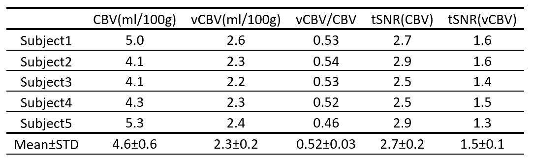
The CSF T₂ map acquired from one subject is shown in Fig. 2 and the averaged T₂ for cortical CSF was 1500+/-220ms, which is very close to the CSF T2 values measured within subarachnoid space¹³. Thus 1500ms was used for the CSF correction.

vCBV and CBV data were processed following the pipeline illustrated in Fig. 3a. As shown in Fig. 3b, CSF contributed a significant portion to the vCBV difference signal(22%+/-20%) in GM. Figure 4 shows the total CBV and vCBV maps from all subjects after correcting for CSF contamination, together with SIPD , DIR(GM), and tSNR maps. The averaged total CBV, vCBV and tSNR values for GM are listed in Table 1. The averaged vCBV in GM is 2.3+/-0.2 mL/100g while the averaged total CBV in GM is 4.6+/-0.6 mL/100g, both comparable to the literature values¹⁴. Meanwhile, the averaged vCBV/CBV ratio is 0.52+/-0.03 which is close to 0.44 based on the morphological microcirculation model^9,15.

Conclusion

We developed a vCBV quantification method that preserves high venular signal and has reduced sensitivity to the arterial transit time and CSF contamination. The measured vCBV and CBV values are comparable to literature values. Although demonstrated with a 2D single-slice acquisition, this method can be further developed for 3D vCBV mapping by replacing the acquisition from the single-shot to multi-shot EPI or GRASE.

Acknowledgements

No acknowledgement found.

References

1. Yablonskiy DA, Sukstanskii AL, He X. Blood oxygenation level-dependent (BOLD)-based techniques for the quantification of brain hemodynamic and metabolic properties - theoretical models and experimental approaches. NMR Biomed. 2013;26(8):963-986.

2. An H, Lin W. Cerebral oxygen extraction fraction and cerebral venous blood volume measurements using MRI: effects of magnetic field variation. Magn Reson Med. 2002;47(5):958-966.

3. Bulte D, Chiarelli P, Wise R, Jezzard P. Measurement of cerebral blood volume in humans using hyperoxic MRI contrast. J Magn Reson Imaging. 2007;26(4):894-899.

4. Blockley NP, Griffeth VEM, Germuska MA, Bulte DP, Buxton RB. An analysis of the use of hyperoxia for measuring venous cerebral blood volume: Comparison of the existing method with a new analysis approach. Neuroimage. 2013;72:33-40.

5. Bolar DS, Rosen BR, Sorensen AG, Adalsteinsson E. QUantitative Imaging of eXtraction of oxygen and TIssue consumption (QUIXOTIC) using venular-targeted velocity-selective spin labeling. Magn Reson Med. 2011;66(6):1550-1562.

6. Stout JN, Adalsteinsson E, Rosen BR, Bolar DS. Functional oxygen extraction fraction (OEF) imaging with turbo gradient spin echo QUIXOTIC (Turbo QUIXOTIC). Magn Reson Med. 2018;79(5):2713-2723.

7. Lee H, Wehrli FW. Cerebral venous blood volume estimation using velocity-selective spin labeling prepared single-slab three-dimensional turbo spin echo imaging. Proc Intl Soc Mag Reson Med. 2019;27:2726.

8. Guo J, Wong EC. Venous oxygenation mapping using velocity-selective excitation and arterial nulling. Magn Reson Med. 2012;68(5):1458-1471.

9. Liu D, Xu F, Lin DD, van Zijl PCMM, Qin Q. Quantitative measurement of cerebral blood volume using velocity-selective pulse trains. Magn Reson Med. 2017;77(1):92-101.

10. Qin Q, Qu Y, Li W, Liu D, Shin T, Zhao Y, Lin DD, van Zijl PCM, Wen Z. Cerebral blood volume mapping using Fourier-transform–based velocity-selective saturation pulse trains. Magn Reson Med. 2019;81:3544.

11. Qin Q, van Zijl PCMM. Velocity-selective-inversion prepared arterial spin labeling. Magn Reson Med. 2016;76(4):1136-1148.

12. Guo J, Wong EC. Removal of CSF contamination in VSASL and QUIXOTIC using a long TE CSF Scan. Proc 19th Annu Meet ISMRM. 2011:2116.

13. Qin Q. A simple approach for three-dimensional mapping of baseline cerebrospinal fluid volume fraction. Magn Reson Med. 2011;65(2):385-391.

14. Leenders KL, Perani D, Lammertsma AA, Heather JD, Buckingham P, Jones T, Healy MJ, Gibbs JM, Wise RJ, Hatazawa J, Herold S, Beaney RP, Brooks D, Spinks T, Rhodes C, Frackowiak RSJ. Cerebral Blood Flow, Blood Volume and Oxygen Utilization: Normal Values and Effect of Age. Brain. 1990;113(1):27.

15. Sharan M, Popel AS. A compartmental model for oxygen transport in brain microcirculation in the presence of blood substitutes. J Theor Biol. 2002;216(4):479-500.

Figures

Figure 1. a) General pulse train for Fourier-Transform based velocity selective saturation (FT-VSS) and inversion (FT-VSI). b) Mz-velocity response for FT-VSS c) Mz-velocity responses for FT-VSI (blue) and with non-selective inversion (NSI) (red). d) The pulse sequence for vCBV measurement. The total CBV can be measured without arterial-nulling module labeled by green dashed box. e) The simulated magnetization evolution of arterial and venous blood.

Figure 2. The image of the first echo (a) and the estimated CSF T2 map (b) measured for one subject. The calculated CSF T2 of 1.5s was used to correct for residual CSF signal in the vCBV quantification.

Figure 3 a) Pipeline to generate a vCBV map. The residual CSF signal in SI_diff,Echo1 was calculated based on SI_diff,Echo2 with a long TE such that only CSF signal is present. A b factor (=1/e^{-(468-18)ms/T2csf}) is used to compensate the T₂ decay of CSF between the two echoes, with fixed T₂,CSF of 1.5s. b) The histogram showing the voxel-by-voxel contribution of CSF signal in SI_diff at the GM area. In this subject, CSF contributed a significant portion in vCBV difference signal (22%±20%) at the GM area.

Figure 4. a) The proton density map (SI_PD), b) DIR (GM) map, c) Total CBV and vCBV maps and d) the corresponding temporal SNR maps for CBV and vCBV sequence for all five subjects. The image scale for total CBV is double that of vCBV to better show vCBV map.

Table 1. The table for averaged total CBV, vCBV and the ratio between vCBV and CBV in GM for all subjects. The temporal tSNR for CBV and vCBV are also listed.

Proc. Intl. Soc. Mag. Reson. Med. 28 (2020)

1110