1097
Multiband first-pass myocardial perfusion MRI using a slice-low-rank plus sparse model
Changyu Sun1, Austin Robinson2, Christopher Schumann2, Daniel Weller1,3, Michael Salerno1,2,4, and Frederick Epstein1,4
1Biomedical Engineering, University of Virginia, Charlottesville, VA, United States, 2Medicine, University of Virginia, Charlottesville, VA, United States, 3Electrical and Computer Engineering, University of Virginia, Charlottesville, VA, United States, 4Radiology, University of Virginia, Charlottesville, VA, United States
1Biomedical Engineering, University of Virginia, Charlottesville, VA, United States, 2Medicine, University of Virginia, Charlottesville, VA, United States, 3Electrical and Computer Engineering, University of Virginia, Charlottesville, VA, United States, 4Radiology, University of Virginia, Charlottesville, VA, United States
Synopsis
Multiband (MB) excitation and in-plane acceleration of first-pass perfusion imaging has the potential to provide a high aggregate acceleration rate. Our recent slice-SPIRiT work formulated MB reconstruction as a constrained optimization problem that jointly uses in-plane and through-plane coil information and MB data consistency. Here we extend these methods to develop k-t slice-SPARSE-SENSE and k-t slice-L+S reconstruction models. First-pass perfusion data with MB=3 and rate-2 k-t Poisson-disk undersampling were acquired in 6 patients. The slice-L+S reconstruction showed sharper borders and greater contrast than slice-SPARSE-SENSE and had better image quality scores as assessed by two cardiologists.
Purpose
First-pass MRI is widely used to image myocardial perfusion. While three slices are typically acquired1, multiband (MB) and in-plane acceleration methods used together promise an increased number of slices and better heart coverage. We recently developed a MB reconstruction model that combines through-plane coil sensitivity, in-plane coil calibration consistency, and consistency with acquired data for iterative joint estimation of all slices2. For MB excitation and in-plane acceleration, here we further develop k-t slice-SPARSE-SENSE and slice-low-rank plus sparse3 (slice-L+S) reconstructions and apply them to first-pass imaging, including comparisons of the two reconstructions.Theory
The k-t slice-L+S model utilizes in-plane sensitivity maps and through-plane kernel calibration information for MB data consistency, and enforces temporal L+S3. The proposed slice-L+S reconstruction (Figure 1B) is expressed in Equation 1:$$\mathop {\arg \min }\limits_{L,S} {\left\| {H\left( {\begin{array}{*{20}{c}} {{L_1} + {S_1}}\\ {{L_2} + {S_2}}\\ \vdots \\ {{L_{{N_s}}} + {S_{{N_s}}}} \end{array}} \right) - {y_{MB}}} \right\|^2} + {\lambda _L}{\left\| {\begin{array}{*{20}{c}} {{L_1}}\\ {{L_2}}\\ \vdots \\ {{L_{{N_s}}}} \end{array}} \right\|_*} + {\lambda _s}{\left\| {T\left( {\begin{array}{*{20}{c}} {{S_1}}\\ {{S_2}}\\ \vdots \\ {{S_{{N_s}}}} \end{array}} \right)} \right\|_1}, (1)$$
where the operator $$$H$$$ (Figure 1C) is defined as $$$H = PQE$$$, $$$N_s$$$ is the number of MB slices, $$$P_z$$$ is the CAIPIRINHA phase modulation matrix for the $$$z^{th}$$$ slice, $$$F$$$ is the fast Fourier transform, $$$E_z$$$ is the sensitivity map for the $$$z^{th}$$$ slice, $$$y_{MB}$$$ is the MB data, $$${\lambda _L}$$$ is the weight for the low-rank constraint, $$${\lambda _S}$$$ is the weight for the temporal frequency sparse constraint, $$$T$$$ is the temporal sparsity operator, $$$m = \left( {\begin{array}{*{20}{c}} {{m_1}}\\ {{m_2}}\\ \vdots \\ {{m_{{N_s}}}} \end{array}} \right) = \left( {\begin{array}{*{20}{c}} {{L_1} + {S_1}}\\ {{L_2} + {S_2}}\\ \vdots \\ {{L_{{N_s}}} + {S_{{N_s}}}} \end{array}} \right)$$$ represents concatenated $$$N_s$$$ coil-combined images undergoing reconstruction as $$$L+S$$$ for all slices, $$$m_z$$$ is the coil-combined image4 of the $$$z^{th}$$$ slice, $$$L = \left( {\begin{array}{*{20}{c}} {{L_1}}\\ {{L_2}}\\ \vdots \\ {{L_{{N_s}}}} \end{array}} \right)$$$, $$$S = \left( {\begin{array}{*{20}{c}} {{S_1}}\\ {{S_2}}\\ \vdots \\ {{S_{{N_s}}}} \end{array}} \right)$$$, $$$P = \left( {{P_1},{P_2},...,{P_{{N_s}}}} \right)$$$, $$$Q = \left( {\begin{array}{*{20}{c}} F& \cdots &0\\ \vdots & \ddots & \vdots \\ 0& \cdots &F \end{array}} \right)$$$ and $$$E = \left( {\begin{array}{*{20}{c}} {{E_1}}& \cdots &0\\ \vdots & \ddots & \vdots \\ 0& \cdots &{{E_{{N_s}}}} \end{array}} \right)$$$.
We use variable splitting5 to decompose the problem into two subproblems: 1) the MB data consistency subproblem written as $$$\mathop {\arg \min }\limits_{{m_1},{m_2},...{m_{{N_s}}}} {\left\| {Hm - {y_{MB}}} \right\|^2} + {\mu ^2}{\left\| {m - \widehat m} \right\|^2}$$$, and 2) the slice-L+S subproblem written as $$$\mathop {\arg \min }\limits_{{{\widehat m}_1},{{\widehat m}_2},...{{\widehat m}_{{N_s}}}} {\lambda _L}{\left\| L \right\|_*} + {\lambda _S}{\left\| TS \right\|_1} + {\left\| {m - \widehat m} \right\|^2}$$$. Here, $$${\mu ^2}$$$ was empirically chosen as 0.4.
We define the conjugate of $$$H$$$ as $$${H^*} = {E^*}{Q^*}{P^*}$$$ (Figure 1D) and redefine $$${Q^*} = \left( {\begin{array}{*{20}{c}} {{F^{ - 1}}{K_1}}& \cdots &0\\ \vdots & \ddots & \vdots \\ 0& \cdots &{{F^{ - 1}}{K_{{N_s}}}} \end{array}} \right)$$$, where $$$K_z$$$ is a matrix that performs a convolution using the split slice-GRAPPA kernel (SP-SG)6.
For comparison, a k-t slice-SPARSE-SENSE method (Figure 1A) using the temporal total variation7 (TV) as a constraint is formulated in Equation 2:
$$\mathop {\arg \min }\limits_{{m_1},{m_2},...{m_{{N_s}}}} {\left\| {H\left( {\begin{array}{*{20}{c}} {{m_1}}\\ {{m_2}}\\ \vdots \\ {{m_{{N_s}}}} \end{array}} \right) - {y_{MB}}} \right\|^2} + {\lambda _1}{\left\| {T\left( {\begin{array}{*{20}{c}} {{m_1}}\\ {{m_2}}\\ \vdots \\ {{m_{{N_s}}}} \end{array}} \right)} \right\|_1} , (2)$$
where $$${\lambda _1}$$$ is empirically chosen as 0.01.
Methods
A saturation-recovery gradient-echo sequence was modified to use MB excitation with CAIPIRINHA8 phase modulation and Poisson-disk k-t undersampling. Imaging was performed on a 1.5T system (Aera, Siemens) using 20-34 receiver channels. Single-band calibration data were acquired in the first heartbeat, and were used to calibrate SP-SG kernels and in-plane sensitivity maps. Six-fold aggregate acceleration was achieved using MB=3 and rate-2 (R=2) k-t undersampling. We implemented slice-SPARSE-SENSE and slice-L+S methods in MATLAB, both based on SP-SG and MB CG-SENSE9, where slice-SPARSE-SENSE used temporal TV compressed sensing6, and slice-L+S used low-rank and temporal-frequency sparsity and were solved using CG10,11 and soft thresholding with variable splitting4. The methods were evaluated in six patients, with 9 slices per patient. The two reconstruction methods were scored (1-5, 5 is best) by two cardiologists.Results
2DIFFT-reconstructions illustrate the artifacts associated with MB=3 and R=2 sampling (Figure 2a), and initial SP-SG reconstructions with remaining R=2 undersampling and slice-separation artifacts are shown in Figure 2b. Example images demonstrating the slice-L+S method are shown in Figure 2c, showing simultaneous decomposition of background and dynamic components for multiple slices. Subsequently, the superposition of L and S demonstrates slice separation and artifact removal (Figure 2d). The example (Figure 3A) compares slice-SPARSE-SENSE and slice-L+S, where slice-L+S shows sharper borders and greater contrast. The cardiologist scoring results were 3.8 ± 0.58 and 4.1 ± 0.36 for slice-SPARSE-SENSE and slice-L+S, respectively (Figure 3B). Figure 4 shows a slice-L+S example of nine-slice coverage.Discussion
We developed slice-SPARSE-SENSE and slice-L+S reconstructions that use through-plane and in-plane coil information, consistency with the acquired data and that enforce temporal constraints. CAPIRINHA phase modulation (MB=3), Poisson-disk (R=2) undersampling and proposed reconstructions provide an effective means to acquire and reconstruct MB first-pass perfusion images. Slice-L+S provides sharper borders and greater contrast than slice-SPARSE-SENSE with temporal TV, though more studies need to be performed. These methods enable the acquisition of nine slices in the time typically required to acquire three slices.Acknowledgements
This work was supported by R01HL147104 and R01HL131919.References
1. Kramer et al. JCMR. 2013;15:19. 2. Sun et al. MRM.2019; DOI:10.1002/mrm.28002. 3. Otazo et al. MRM, 2015; 73(3): 1125-1136. 4. Uecker et al. MRM, 2014; 71(3): 990-1001. 5. Huang et al. MRM, 2010; 64(4): 1078-1088. 6. Cauley et al. MRM.2014; 72(1):93-102. 7. Feng et al. MRM, 2014; 72(3): 707-717. 8. Breuer et al. MRM, 2005; 53(3): 684-691. 9. Yutzy et al. MRM, 2011; 65(6): 1630-1637. 10. Lustig et al. MRM, 2010, 64: 457-471. 11. Paige et al. TOMS, 1982, 8: 43-71.Figures
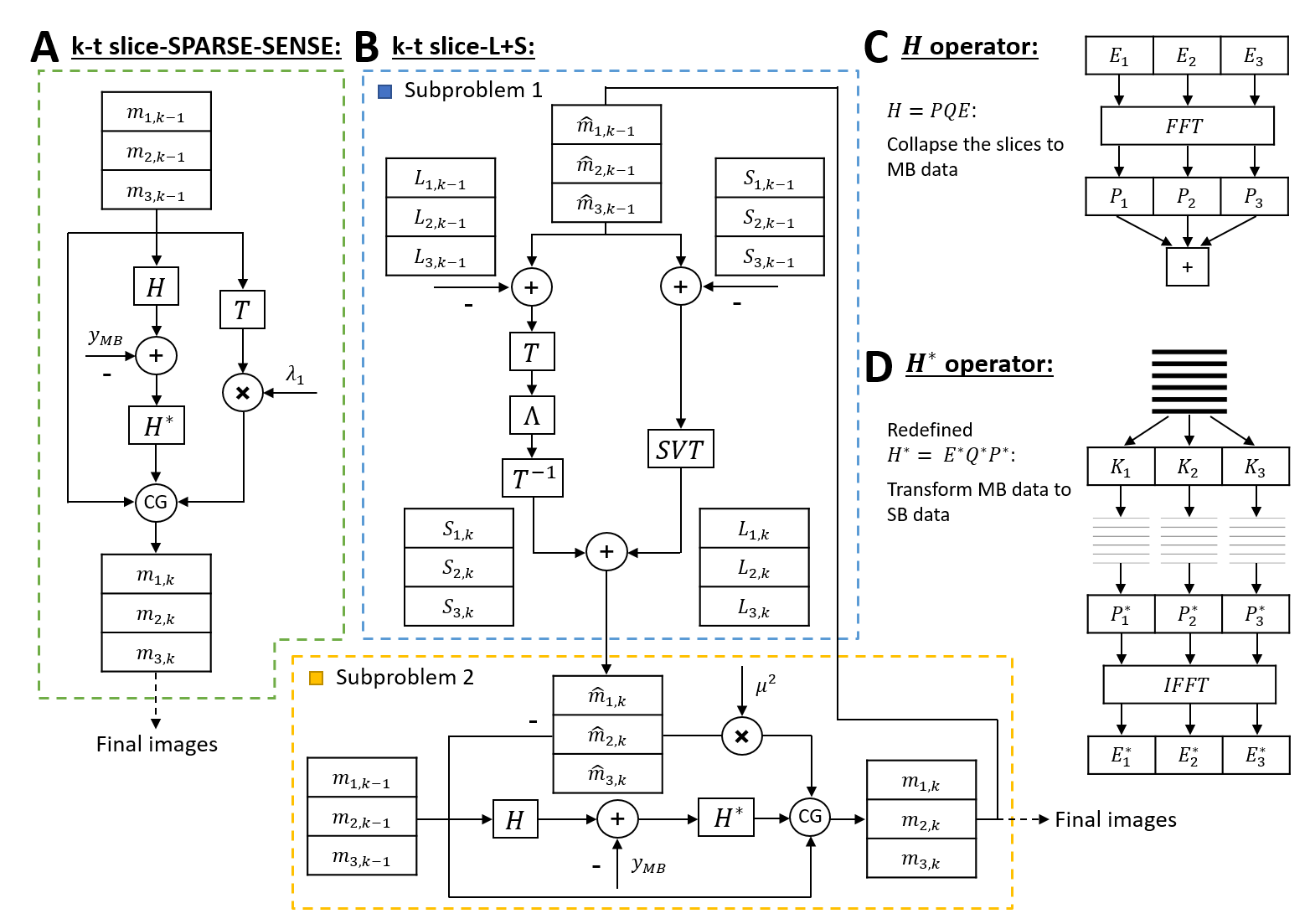
Figure 1: A: The solution of the k-t slice-SPARSE-SENSE
model using CG. B: The solution of the k-t slice-L+S model using CG and
soft-thresholding with variable splitting. Λ is the temporal sparsity
thresholding and SVT is the singular value
thresholding. C: the H operator is
depicted, including use of sensitivity maps (E), FFT (F), phase modulation (P)
and summation. D: The approximation of H* is depicted, including
slice-separating K kernels, phase demodulation (P*), IFFT (F-1)
and coil combination (E*).
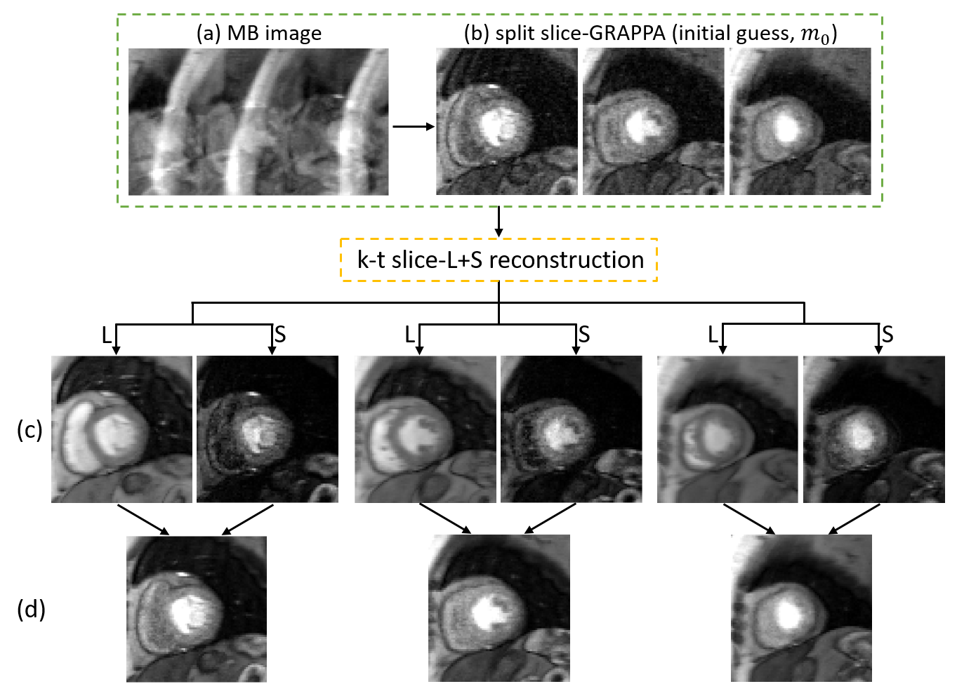
Figure 2: Rate-6 accelerated perfusion imaging with MB=3
and in-plane undersampling with R=2. 2DIFFT-reconstructions illustrate the artifacts associated with MB=3 and
R=2 sampling (a). Three slices separated using split slice-GRAPPA show remaining
in-plane undersampling artifacts and slice separation artifacts, and form the
initial guess for k-t slice-L+S (b). Images reconstructed by k-t slice-L+S
demonstrate background (L) and dynamic (S) components of three slices simultaneously
(c). The superposition of L and S demonstrates slice separation and artifact
removal (d).
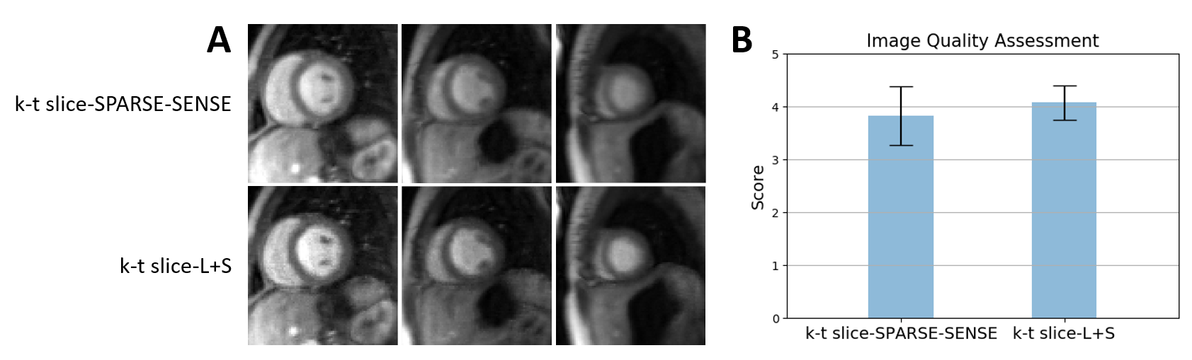
Figure 3: A: Comparison of k-t slice-SPARSE-SENSE
using temporal TV and k-t slice-L+S for image reconstruction applied to first-pass
perfusion MRI with MB=3 and in-plane undersampling with R=2 (three short-axis
slices from a patient are shown). Slice-L+S shows sharper borders and greater
contrast compared to k-t slice-SPARSE-SENSE. B: Blinded image-quality scores
for all 6 subjects. The bar plot shows the mean score of slice-L+S is higher than
slice-SPARSE-SENSE with lower standard deviation.
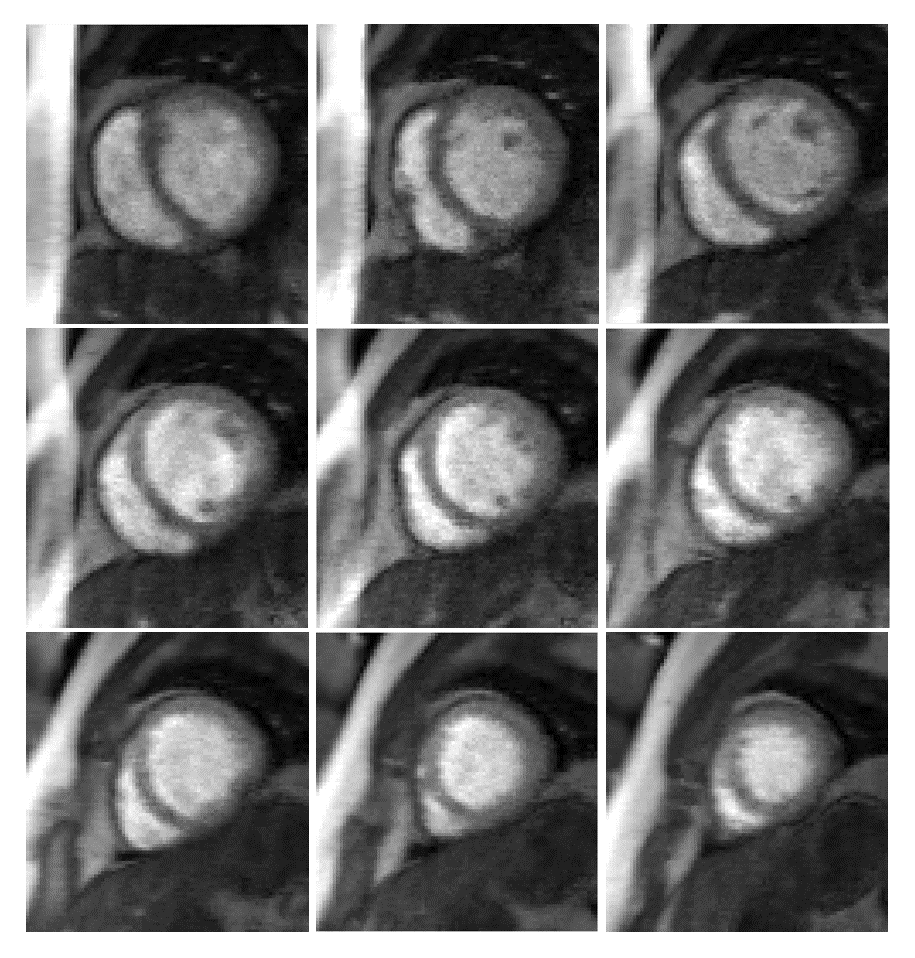
Figure 4: Rate-6 accelerated perfusion images with
MB=3 and in-plane undersampling with R=2 provides 9-slice coverage using k-t slice-L+S.