Introduction

Time-resolved 3D phase-contrast Magnetic Resonance Imaging (or 4D Flow MRI) is a promising tool for in-vivo non-invasive blood flow quantification. As it relies on complex physical principles and multimodal acquisition, different types of velocity measurement errors arise, which can impair diagnosis. Numerical simulation of the MRI acquisition process enables to reconstruct synthetic images free of experimental errors in order to identify their origins. Although many simulation frameworks have been developed for static tissues imaging^1,2, flow MRI modeling remains challenging mainly because of the need to account for the spin dynamics, which results in noticeable increase in computational load. The objective of this work is to present a 4D flow MRI simulation workflow of a realistic pulsatile flow typical of the cardiovascular system.

Methods

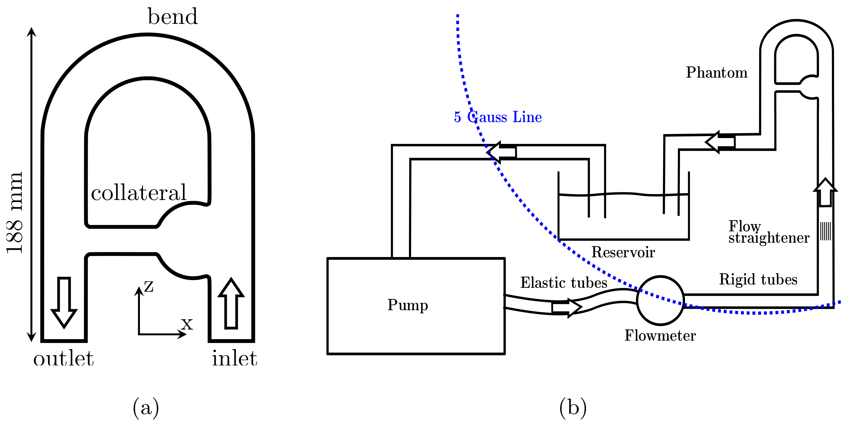
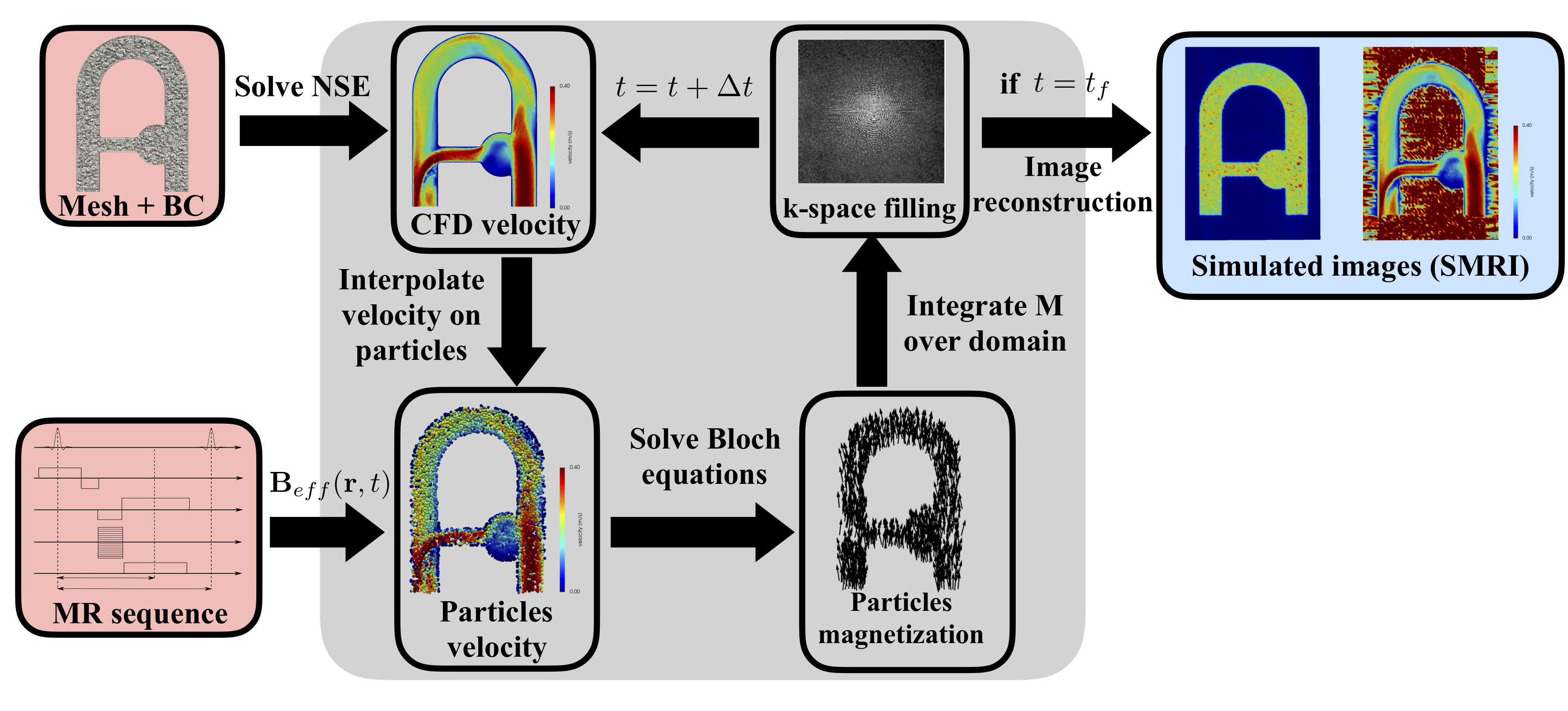
We designed a well-controlled experiment delivering pulsatile blood-mimicking fluid flow within a rigid phantom and carried out PC-MRI experiments. An image-based CFD analysis was performed from the PC-MRI data prescribed as inlet velocity profile³. The Bloch equations were solved at each iteration and the spin positions updated “on the fly” from CFD velocity hence eliminating the need to store particles trajectories. The experimental setup is depicted in figure 1.

Simulation of flow MR imaging (illustrated in figure 2): N_p particles are injected with a uniform random distribution into each cell of a fixed unstructured numerical mesh. At each iteration, the Navier-Stokes equations are solved on the unstructured mesh using YALES2BIO solver⁴. The CFD velocity was interpolated on each particle to update their position. Each particle is associated with magnetic properties (T1, T2, M₀), an isochromat volume, and an injection magnetization M_inj = (0, 0, M_z^ss) where M_z^ss is the steady state magnetization. At each spoiling event, particles are suppressed and N_p particles are reinjected at the same location as initially. This key step of the methodology allows to keep the particles distribution homogeneous and avoid spurious-signal areas. An effective magnetic field imposed by the (idealized) MR sequence designed with JEMRIS² was prescribed to each particle at each instant. From a multi-criterion time-stepping approach, the magnetization vector was either advanced with a full numerical integration (4th-order Runge-Kutta) of the Bloch equations whenever the Radio-Frequency field (RF) is on, or by the analytical solution (given that the gradient waveform can be analytically described.
MR parameters: A RF-spoiled time-resolved 3D Gradient echo sequence with three velocity encoding gradients was simulated. A 2 mm³ voxel size was set with a flip angle =15°, TR=6 ms, ∆T = 58 ms, and a VENC_x,y,z=60 cm/s.

Reconstruction: The resulting MR signal was Fourier-transformed in order to reconstruct synthetic MR images and velocity field. As the simulated MR images are stripped of experimental errors, the sources of observed discrepancies can be better highlighted.

Validation: The simulated MR velocity field (u_SMRI) was compared with the phase-averaged CFD velocity fields (u_CFD) to validate the CFD coupling. Prior to the comparison, CFD velocity field were downsampled to the MRI spatial resolution. In addition, u_SMRI was compared to 4D Flow MR measurements (u_MRI) to identify the major discrepancy sources.

Results

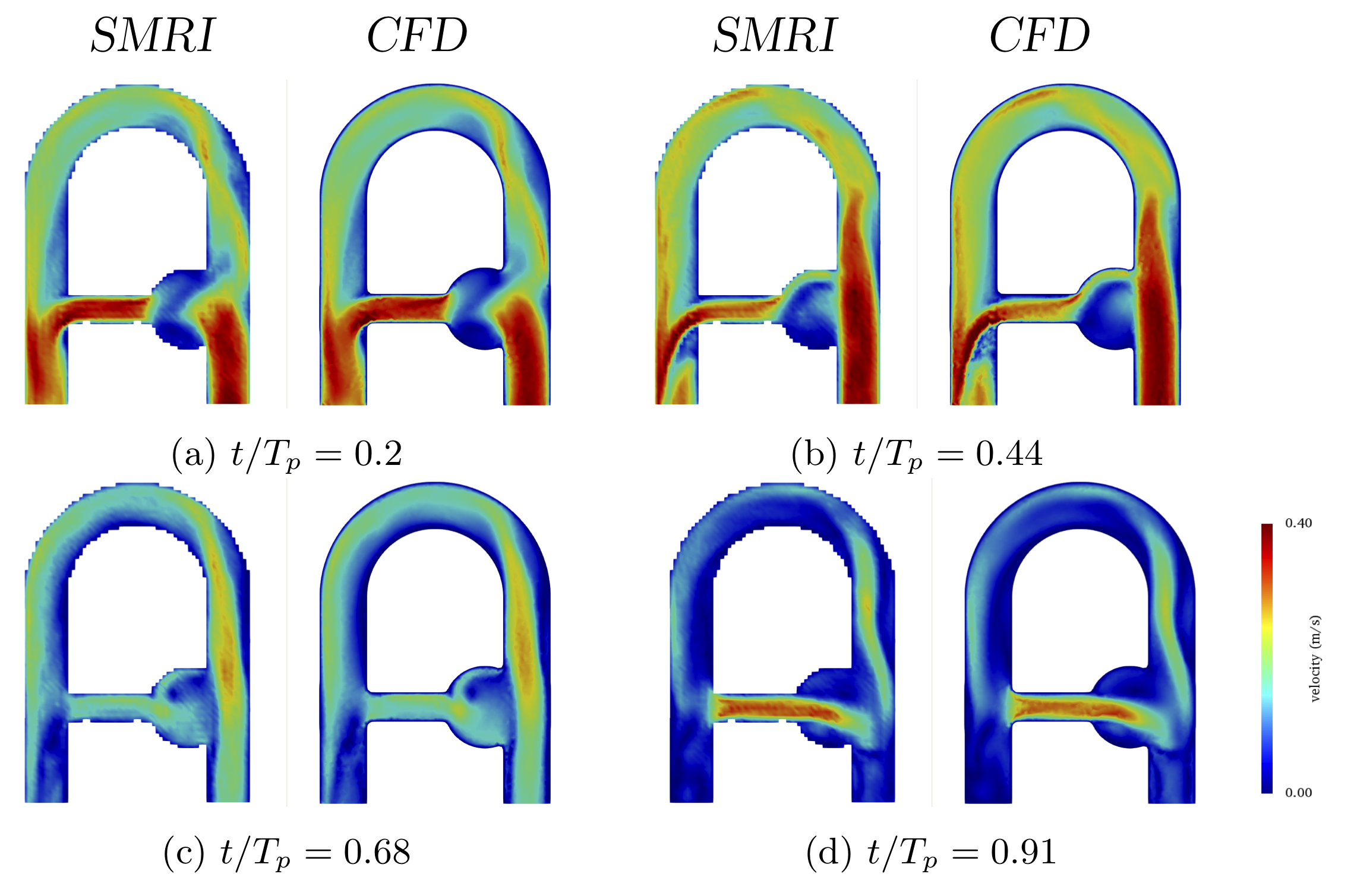
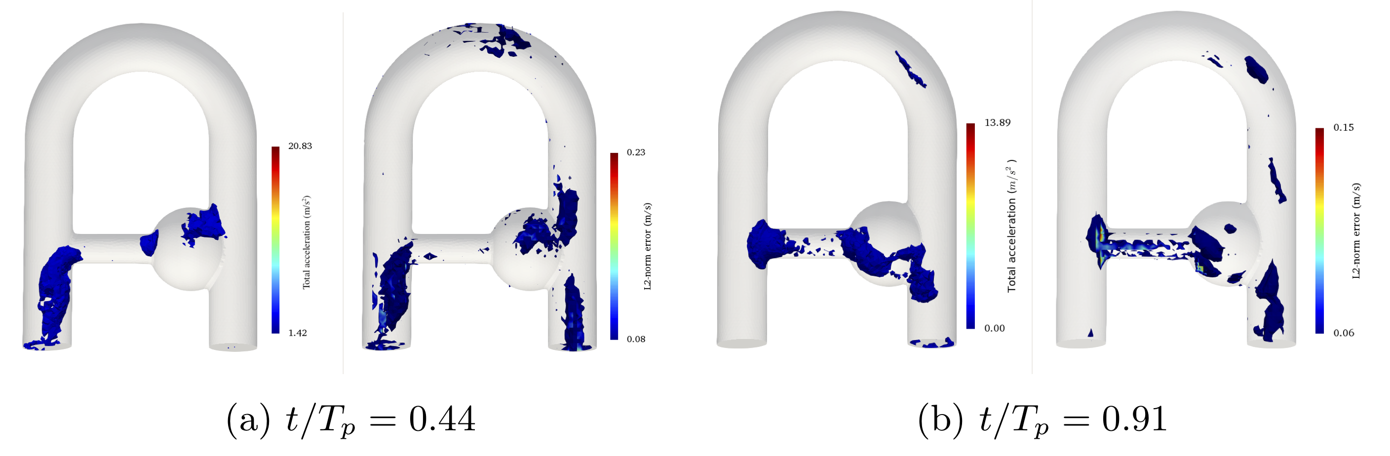
Figure 3 shows excellent agreement between imposed u_CFD and u_SMRI regardless of the phase (peak and mean correlation coefficients: r² = 0.978 and 0.966). While the MRI simulation suppresses many sources of discrepancies, some still remain such as misregistration artifacts, intravoxel phase dispersion, Gibbs artifacts or velocity fluctuations effects.
To identify the largest velocity error contribution, the highest error patterns were compared to the highest CFD acceleration patterns in figure 4. The high visual correlation confirms that acceleration-induced artifacts contribute for the main errors. Note also that the sparse particles distribution near the inlet boundary induces high velocity error.
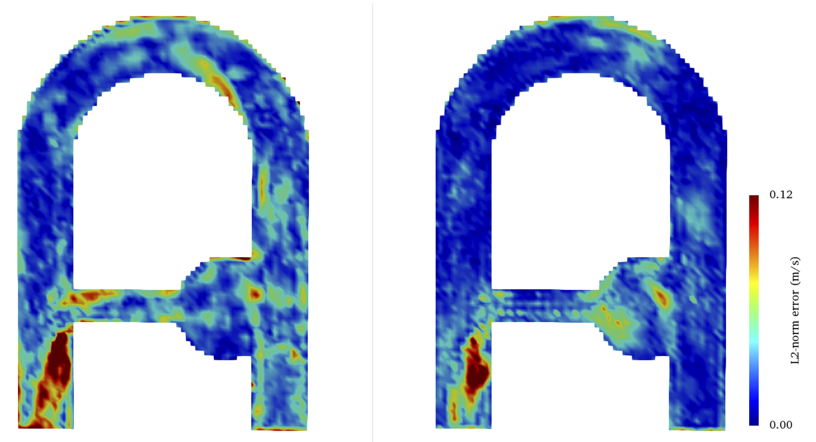
The velocity error produced by MRI simulation with respect to CFD was qualitatively compared to the error raised between MR measurements (u_MRI) and CFD in figure 5. Generally speaking, a good agreement and reproducible error patterns are generally noticed with a net error decrease in u_SMRI. It is suggested that the highest error site located at the collateral elbow (and well reproduced by the simulation) is the result of both misregistration artifacts and intravoxel dispersion.

Discussion

In this study, we presented a workflow for simulating realistic 4D flow MR acquisitions. Several coupled CFD-MRI simulations of a well-controlled flow phantom experiment were performed and compared to the phase-averaged CFD velocity. Reported at peak systole, the largest velocity discrepancies were mainly located in the regions of high flow acceleration. It was suggested that these errors appear since the particle acceleration is not accounted for in the phase-velocity relationship. Acceleration-sensitive acquisitions could be carried out to account for the flow high-order motion⁵ or pre-processing corrections could be applied to the velocity field⁶. The experimental MRI was also compared to the simulated MRI and similar error patterns were reported as compared to the CFD, were small rotating structures and high convective acceleration induce image artifacts. However, some unquantified errors still arise because of the differences between experimental and simulated MR sequences. A crucial step to compare MRI simulation to MRI measurements is to simulate the same MR sequence as the one applied experimentally. This work constitutes a preliminary phase to further exploit the MRI simulation capabilities.

Acknowledgements

No acknowledgement found.