1034

In vivo voxel-wise parcellation of the human cerebral cortex using 3D MR fingerprinting (MRF) and supervised machine learning classification

Shahrzad Moinian¹, Viktor Vegh^1,2, and David Reutens^1,2
¹Centre for Advanced Imaging, The University of Queensland, Brisbane, Australia, ²ARC Centre for Innovation in Biomedical Imaging Technology, The University of Queensland, Brisbane, Australia

Synopsis

The human cerebral cortex may be divided into functionally different, microarchitectonically distinct areas. While quantitative multi-modal MRI methods can reveal microstructural characteristics of cortical tissue, accurate microarchitectural parcellation of the entire cortex is yet to be attained. Here, we examine a novel method of automated in vivo voxel-wise cortical parcellation which exploits the area-specific microstructural information present in MR fingerprinting (MRF) signals. A Radial Basis Function Support Vector Machine (RBF-SVM) classifier, trained with a volume-based feature representation, achieved a macro-average area under the Receiver Operating Characteristic curve (ROC-AUC) of 0.83.

Introduction

Accurate architectonic parcellation of the human cerebral cortex may enable better understanding of the brain function.¹ While quantitative histology-based methods provide accurate microstructural cortical maps,² they are not directly translatable to the individual humans, and the most promising in vivo quantitative MR-based microstructural cortical mapping methods are yet to achieve sufficient accuracy.^3,4 We previously described an MR Fingerprinting (MRF) method which distinguished between three cortical areas (BA2: primary somatosensory cortex, BA4: primary motor cortex and BA6: premotor cortex). Particularly, we demonstrated the presence of information in MRF signals complementary to MR relaxometry, a potentially useful finding for accurate in vivo human cortical parcellation.⁵ Subsequently, we employed supervised machine learning classification and showed feasibility of using the voxel-wise MRF residual signals for automating the in vivo voxel-wise parcellation of BA2, BA4 and BA6.⁶ The main drawbacks of the method were i) limited cortical coverage, and ii) low SNR, resulted from the use of a 2D EPI-based⁷ MRF sequence for MRF acquisitions. Here, we aimed to extend the utility of the automatic voxel-wise cortical parcellation method through a 3D MRF sequence.

Methods

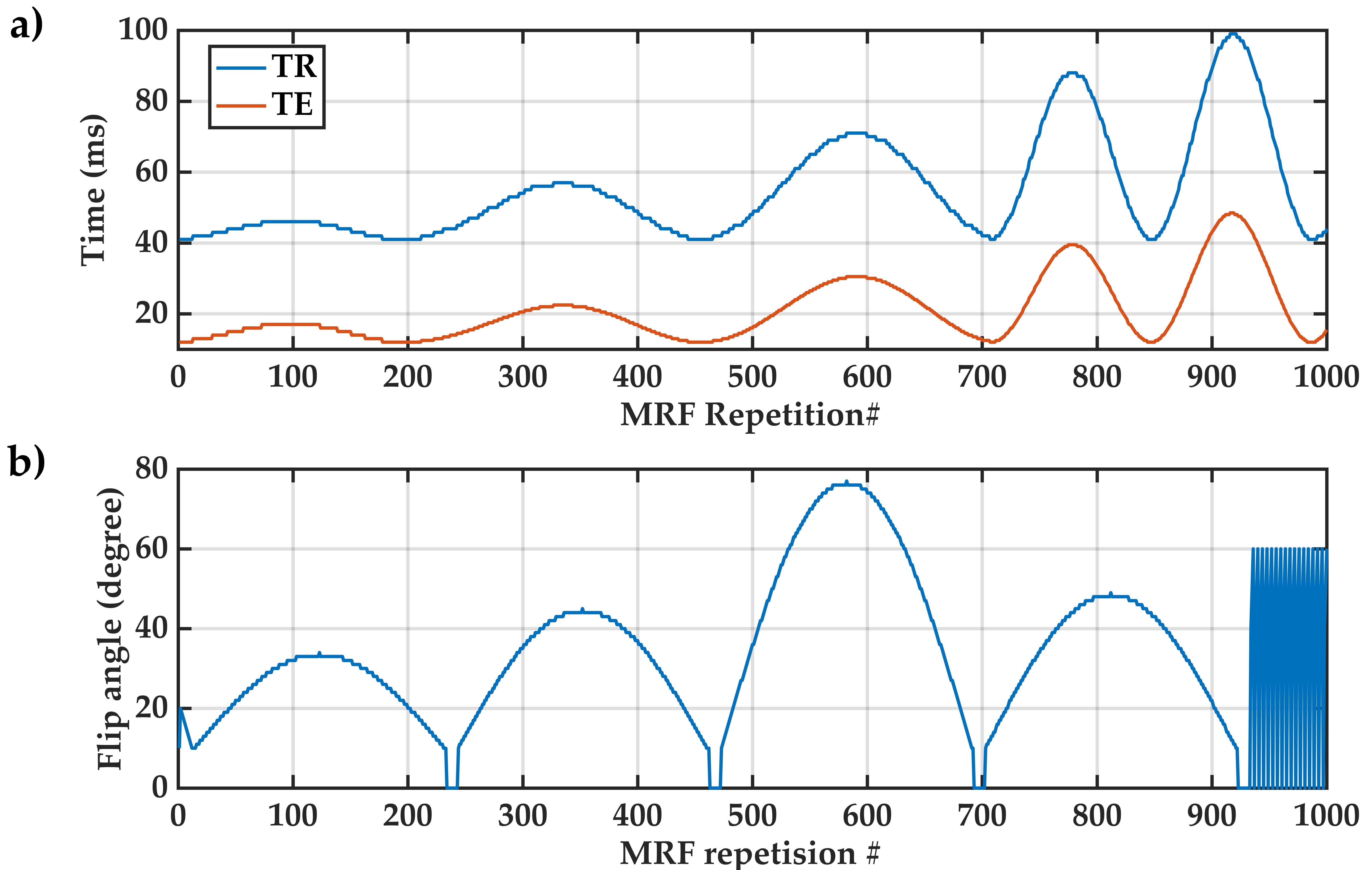
We scanned six healthy participants aged between 27 and 35 years using a 3D EPI-based⁸ MRF sequence developed in-house on a 7T whole-body MRI research scanner (Siemens Healthcare, Erlangen, Germany). MRF parameters were as follows: 1000 frames of 3D MRF images, TR=41-99ms (Figure 1a), TE=12-48ms (Figure 1a),⁹ FA=10-77° (Figure 1b),¹⁰ Partial Fourier Phase=6/8, voxel size=1.4×1.4×1.4mm³, matrix size=142×142×88, and GRAPPA parallel imaging¹¹ in phase (acceleration=3; reference lines=36) and slice encoding (acceleration=2; reference lines=12) directions. Each MRF scan was performed twice in two separate sessions to boost SNR via averaging.
We acquired a 3D B1⁺map (SA2RAGE¹²) for B1⁺ inhomogeneity correction of MRF signals.¹³ The voxels of interest from primary somatosensory cortex BA1 and BA2, primary motor cortex BA4a, premotor cortex BA6, visual cortex BA17 and BA18, and Broca area BA45 were extracted from the Juelich histological human brain atlas,^14,15 after FNIRT¹⁶ transformation from MNI to MRF space. For each voxel of interest, we calculated the MRF residual signal as the difference between the acquired MRF signal and its best match from an MRF dictionary. A voxel-wise feature vector was formed as previously described,⁶ using a set of 999 normalised MRF residual signal autocorrelations. Feature vectors were pre-processed as: 1) feature selection through MRF residual signal under-sampling at every n^th acquisition, 2) min-max feature scaling, and 3) Neighbourhood Component Analysis (NCA) feature extraction.¹⁷ We applied random over-sampling (ROS) for the class imbalance problem,¹⁸ then formulated the parcellation of the seven target cortical areas as a multi-class classification problem, and uniquely labelled feature vectors of each cortical area. Through a grid search¹⁹ 5-fold cross-validation²⁰ model selection procedure, we compared the prediction performance of linear support vector machine (Linear-SVM), Radial Basis Function SVM (RBF-SVM), Random Forest and K-nearest neighbours (KNN) supervised classification algorithms using two different feature representation approaches: i) features from MRF residual of each voxel, and ii) features derived from the average MRF residuals of a volume comprising 3×3×3 voxels, centred at the target voxel.

Results and Discussion

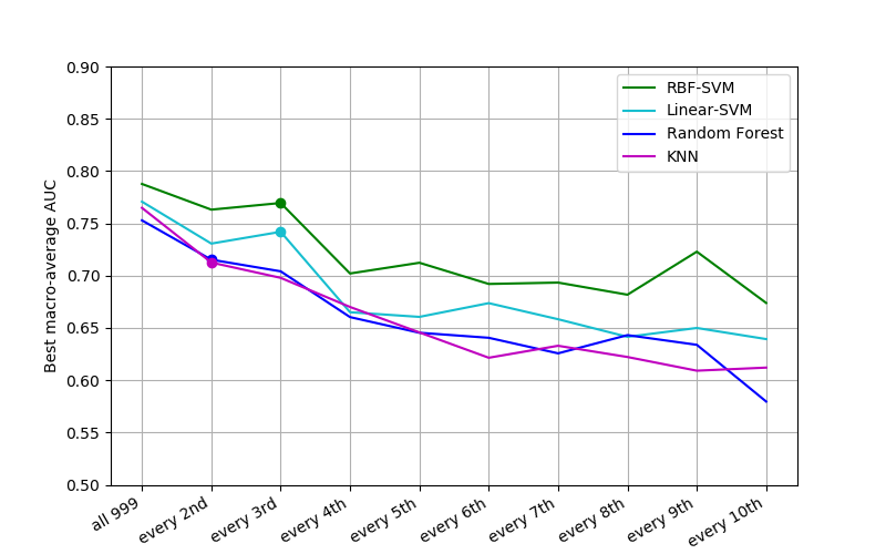
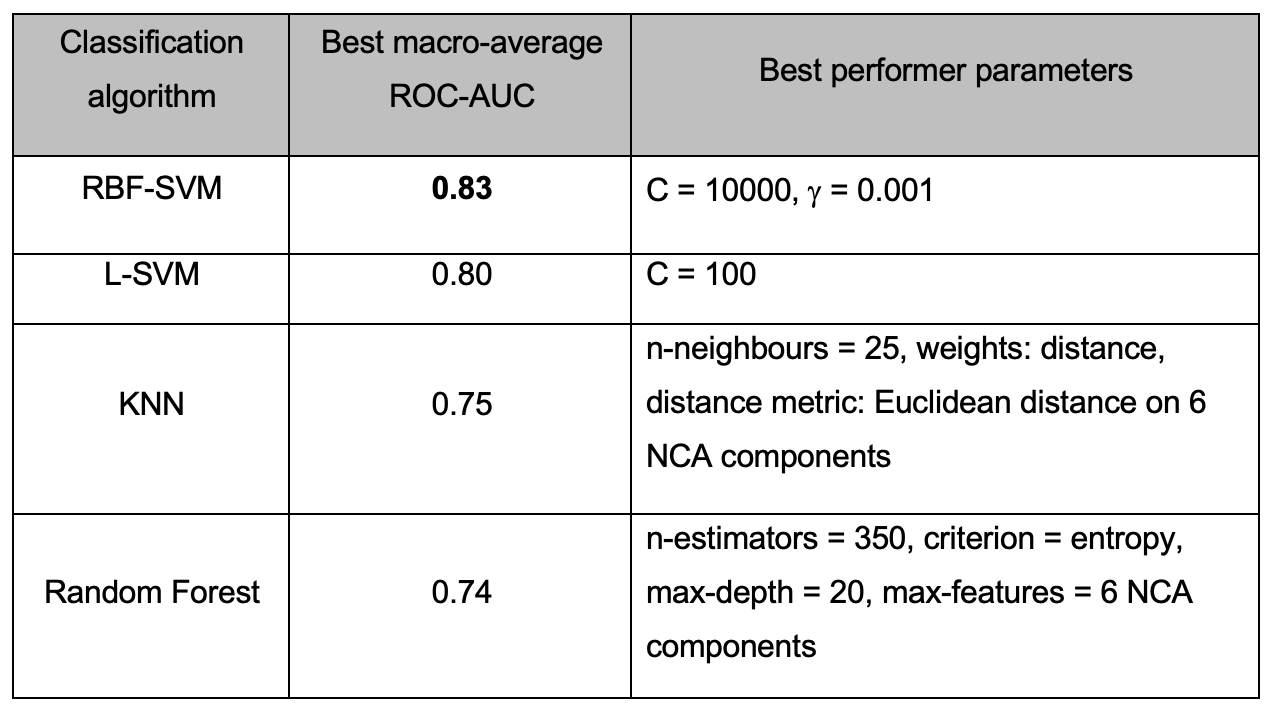
The horizontal axis for the feature and model selection results shown in Figure 2 illustrates the feature selection steps, leading to inclusion of a different feature subset in the model selection process. RBF-SVM (with regularisation parameter C=1000 and kernel parameter γ=0.001) was found to perform best, with macro-average area under the Receiver Operating Characteristic curve (ROC-AUC) of 0.79 for class predictions of the held-out test set.
Figure 3 details the model selection process using the volume-based feature representation approach. The RBF-SVM model (C=10000, γ=0.001) outperformed all other models investigated, with macro-average ROC-AUC of 0.83 (sensitivity of 0.71, specificity of 0.95).
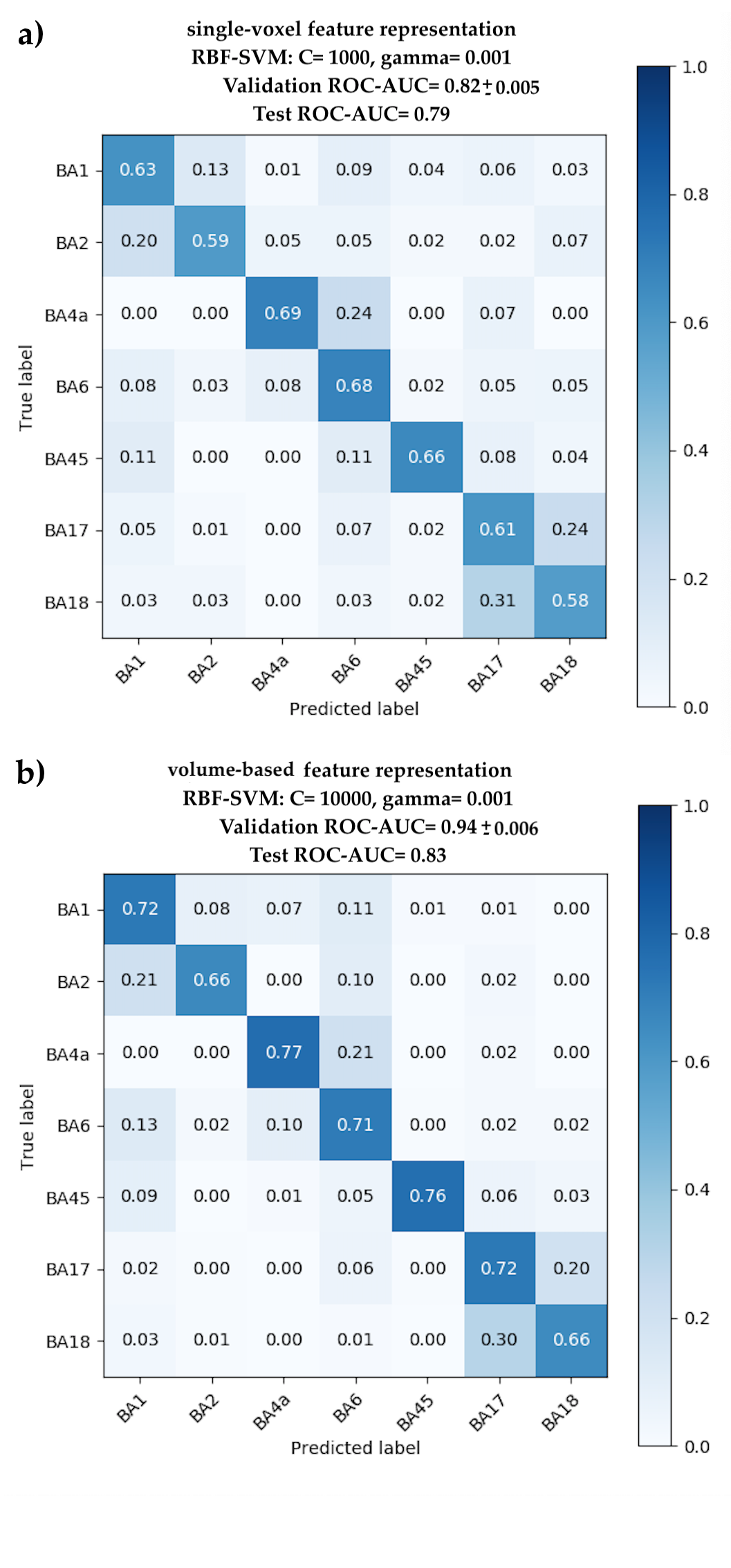
We found the ROC-AUC of predictions on the held-out test set was improved by using the volume-based feature representation (Figure 4; ROC-AUC increases to 0.83 from 0.79). The higher prediction accuracy of volume-based feature representation may stem from its hybrid local-global parcellation approach, and is in line with similar improvements observed in other hybrid cortical mapping methods.²¹ Moreover, the false negative rates (FNR) along each row (excluding diagonal values) of the confusion matrix of the best classifier (Figure 4b) may imply microstructural similarities between the cortical areas of interest. For example, when comparing the similarity of BA2, BA4a and BA6, out of all the data samples of BA2, 10% were incorrectly predicted as BA6, and none as BA4a, suggesting higher dissimilarity between the features of BA2 and BA4a than between BA2 and BA6. These findings agree with the microstructural similarity measurements between these three areas as reported by others.^22,23
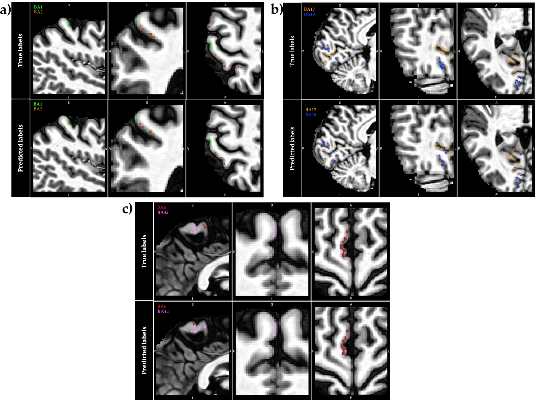
Figure 5 depicts a representative distribution of the true class (top panels) versus the predicted labels (bottom panels) for the held-out test set, using the selected RFB-SVM classifier trained with the volume-based feature vectors (Figure 4b).

Conclusions

We have demonstrated the feasibility of automatic, in vivo, voxel-wise parcellation of seven cortical areas, using a 3D EPI-MRF sequence. We found improved prediction performance when using a volume-based feature representation, instead of using features from a single voxel. Future work may involve extending the method towards whole cortex parcellation.

Acknowledgements

The authors acknowledge the facilities and scientific and technical assistance of the National Imaging Facility, a National Collaborative Research Infrastructure Strategy (NCRIS) capability, at the Centre for Advanced Imaging, The University of Queensland. We also thank Nicole Atcheson and Aiman Al Najjar from the Centre for Advanced Imaging, The University of Queensland for helping with the MRI data acquisition.

References

1. Honey CJ, Thivierge JP, Sporns O. Can structure predict function in the human brain? Neuroimage. 2010;52(3):766-76.

2. Schleicher A, Amunts K, Geyer S, Morosan P, Zilles K. Observer-independent method for microstructural parcellation of cerebral cortex: A quantitative approach to cytoarchitectonics. Neuroimage. 1999;9(1):165-77.

3. Cercignani M, Bouyagoub S. Brain microstructure by multi-modal MRI: Is the whole greater than the sum of its parts? Neuroimage. 2018;182:117-27.

4. Edwards LJ, Kirilina E, Mohammadi S, Weiskopf N. Microstructural imaging of human neocortex in vivo. Neuroimage. 2018;182:184-206.

5. Moeiniyan Bagheri S, Vegh V, Reutens D. Magnetic Resonance Fingerprinting (MRF) can reveal microstructural variations in the brain gray matter. ISMRM; Paris2018.

6. Moeiniyan Bagheri S, Vegh V, Reutens D. Towards in-vivo voxel-wise parcellation of human brain cortex. ISMRM; Montreal2019.

7. Turner R, Le Bihan D, Maier J, Vavrek R, Hedges LK, Pekar J. Echo-planar imaging of intravoxel incoherent motion. Radiology. 1990;177(2):407-14.

8. Poser BA, Koopmans PJ, Witzel T, Wald LL, Barth M. Three dimensional echo-planar imaging at 7 Tesla. Neuroimage. 2010;51(1):261-6.

9. Rieger B, Zimmer F, Zapp J, Weingartner S, Schad LR. Magnetic Resonance Fingerprinting Using Echo-Planar Imaging: Joint Quantification of T-1 and T-2* Relaxation Times. Magnetic Resonance in Medicine. 2017;78(5):1724-33.

10. Buonincontri G, Sawiak SJ. MR Fingerprinting with Simultaneous B1 Estimation. Magnetic Resonance in Medicine. 2016;76(4):1127-35.

11. Griswold MA, Jakob PM, Heidemann RM, Nittka M, Jellus V, Wang J, et al. Generalized autocalibrating partially parallel acquisitions (GRAPPA). Magn Reson Med. 2002;47(6):1202-10.

12. Eggenschwiler F, Kober T, Magill AW, Gruetter R, Marques JP. SA2RAGE: a new sequence for fast B1+ -mapping. Magn Reson Med. 2012;67(6):1609-19.

13. Ma D, Coppo S, Chen Y, McGivney DF, Jiang Y, Pahwa S, et al. Slice profile and B1 corrections in 2D magnetic resonance fingerprinting. Magn Reson Med. 2017;78(5):1781-9.

14. Eickhoff SB, Stephan KE, Mohlberg H, Grefkes C, Fink GR, Amunts K, et al. A new SPM toolbox for combining probabilistic cytoarchitectonic maps and functional imaging data. Neuroimage. 2005;25(4):1325-35.

15. Jülich. Jülich histological (cyto- and myelo-architectonic) atlas references. [Available from: https://fsl.fmrib.ox.ac.uk/fsl/fslwiki/Atlases/Juelich.

16. Andersson JL, Jenkinson M, Smith S. Non-linear registration aka Spatial normalisation FMRIB Technial Report TR07JA2. FMRIB Analysis Group of the University of Oxford. 2007.

17. Goldberger J, Hinton GE, Roweis ST, Salakhutdinov RR, editors. Neighbourhood components analysis. Advances in neural information processing systems; 2005.

18. Batista GE, Prati RC, Monard MC. A study of the behavior of several methods for balancing machine learning training data. ACM SIGKDD explorations newsletter. 2004;6(1):20-9.

19. Hsu C-W, Chang C-C, Lin C-J. A practical guide to support vector classification. 2003.

20. Wong TT. Performance evaluation of classification algorithms by k-fold and leave-one-out cross validation. Pattern Recogn. 2015;48(9):2839-46.

21. Schaefer A, Kong R, Gordon EM, Laumann TO, Zuo XN, Holmes AJ, et al. Local-Global Parcellation of the Human Cerebral Cortex from Intrinsic Functional Connectivity MRI. Cereb Cortex. 2018;28(9):3095-114.

22. Cohen-Adad J, Polimeni JR, Helmer KG, Benner T, McNab JA, Wald LL, et al. T2* mapping and B0 orientation-dependence at 7 T reveal cyto-and myeloarchitecture organization of the human cortex. Neuroimage. 2012;60(2):1006-14.

23. Glasser MF, Van Essen DC. Mapping Human Cortical Areas In Vivo Based on Myelin Content as Revealed by T1- and T2-Weighted MRI. J Neurosci. 2011;31(32):11597-616.

Figures

Figure 1. The pseudo-randomised pattern of a) repetition time (TR) and echo time (TE), and b) flip angles, used to acquire the 3D MRF images.

Figure 2. The best macro-average ROC-AUC scores of four supervised classification algorithms are compared when trained with different subset of autocorrelation values as the feature vectors. The classification methods used here are Linear-SVM (Linear Support Vector Machine), RBF-SVM (Radial Basis Function kernel SVM), RF (Random Forests) and KNN (K-Nearest Neighbours). The solid circle on each plot represents the subset of autocorrelations at which that model showed its best performance, compared to the initial case of including the whole 999 autocorrelation values.

Figure 3. The ROC-AUC scores of four supervised classification methods are compared, when the volume-based approach was used for feature representation of each voxel.

Figure 4. Normalised confusion matrices for the best performer (i.e. RBF-SVM classifier) trained with a) the single-voxel feature representation, and b) the volume-based feature representation. The model parameters, the validation and the test ROC-AUC scores of the best classifier are stated at the top. Cell values along the diagonal represent the sensitivity of the model predictions on the held-out test set. The values were rounded up to two decimal places.

Figure 5. True class labels (top) versus the predicted class labels (bottom) for a) primary somatosensory cortex areas BA1 and BA2, b) visual cortex areas BA17 and BA18, and c) premotor cortex area BA6 and primary motor cortex BA4a of the held-out participant, using the RBF-SVM classifier trained with the volume-based feature representation. The class labels are overlaid on an anatomical image of the participant.

Proc. Intl. Soc. Mag. Reson. Med. 28 (2020)

1034