1033

Improved Depiction of Meningioma Boundaries in MR Elastography Using a Novel Inhomogeneous Learned Inversion

Jonathan M Scott¹, Arvin Arani², Armando Manduca², Joshua D Trzasko², John Huston III², Richard L Ehman², and Matthew C Murphy²
¹Medical Scientist Training Program, Mayo Clinic, Rochester, MN, United States, ²Radiology, Mayo Clinic, Rochester, MN, United States

Synopsis

Magnetic Resonance Elastography stiffness estimates in small focal lesions are often inaccurate. The assumption of material homogeneity made by most inversion algorithms likely contributes to these errors. Here we describe a machine-learning based inversion algorithm trained on wave simulations of materials with piecewise smooth stiffness variations (Inhomogeneous Learned Inversion, ILI). We show that ILI offers improved delineation of tumor boundaries over two inversions assuming material homogeneity in a series of 17 patients with stiff meningiomas.

Introduction

Magnetic Resonance Elastography (MRE) is an MRI-based method for noninvasive assessment of tissue mechanical properties¹. In focal disease, MRE-measured stiffness has been shown to differentiate benign from malignant tumors^2–4and preoperatively characterize intracranial tumor mechanical properties^5,6. While promising, these early studies have excluded small lesions (<2cm in diameter) due to limited spatial resolution^2,3,6. Inversion algorithms, which estimate mechanical properties from acquired displacement data, are one factor limiting the spatial resolution of MRE. Most commonly used inversion algorithms assume homogeneous stiffness^7,8, and those that do not frequently penalize heterogeneity within a region of interest⁹. We previously reported improved spatial resolution in simulation and phantom studies with a machine-learning based inversion algorithm that does not assume local homogeneity¹⁰. However, when moving in vivo this inversion artefactually increased stiffness, likely because it was trained on data of a single fixed damping ratio. Here we describe an updated inversion, Inhomogeneous Learned Inversion (ILI), which is trained on simulations with piecewise smooth stiffness that cover the full range of physiologic damping ratios. We then evaluate ILI in comparison with a previously reported homogeneous learned inversion (HLI)⁷ and direct inversion (DI)¹¹ in a series of stiff meningiomas.

Methods

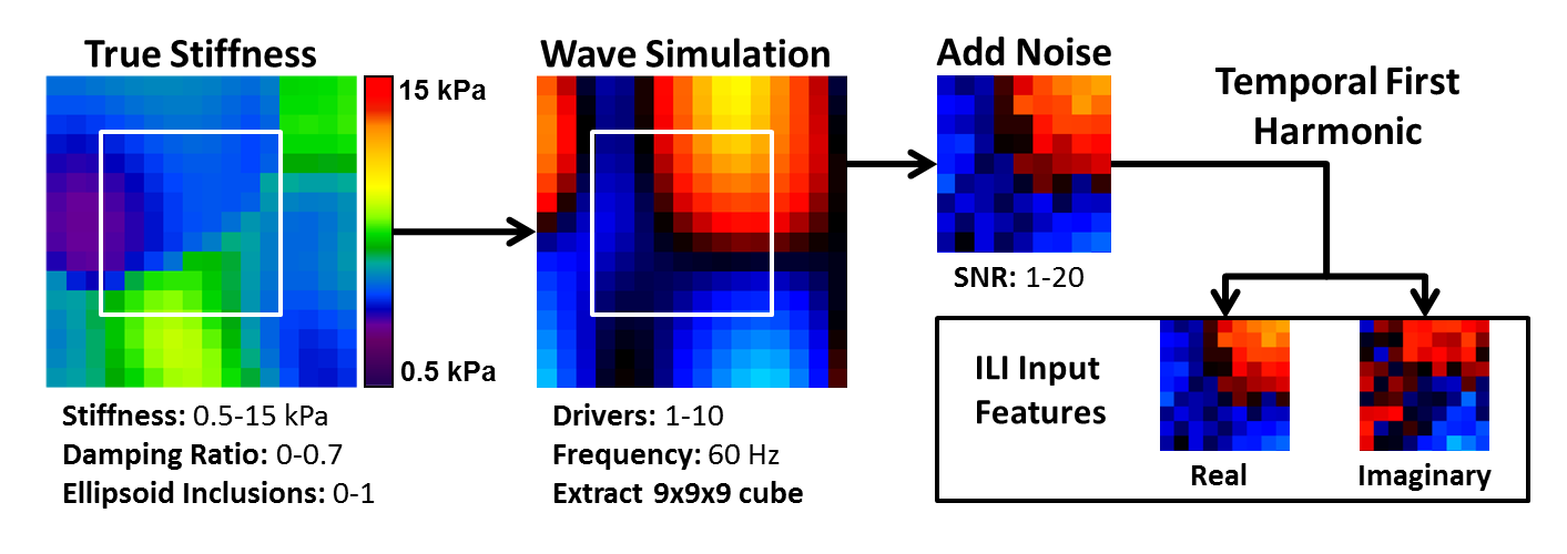
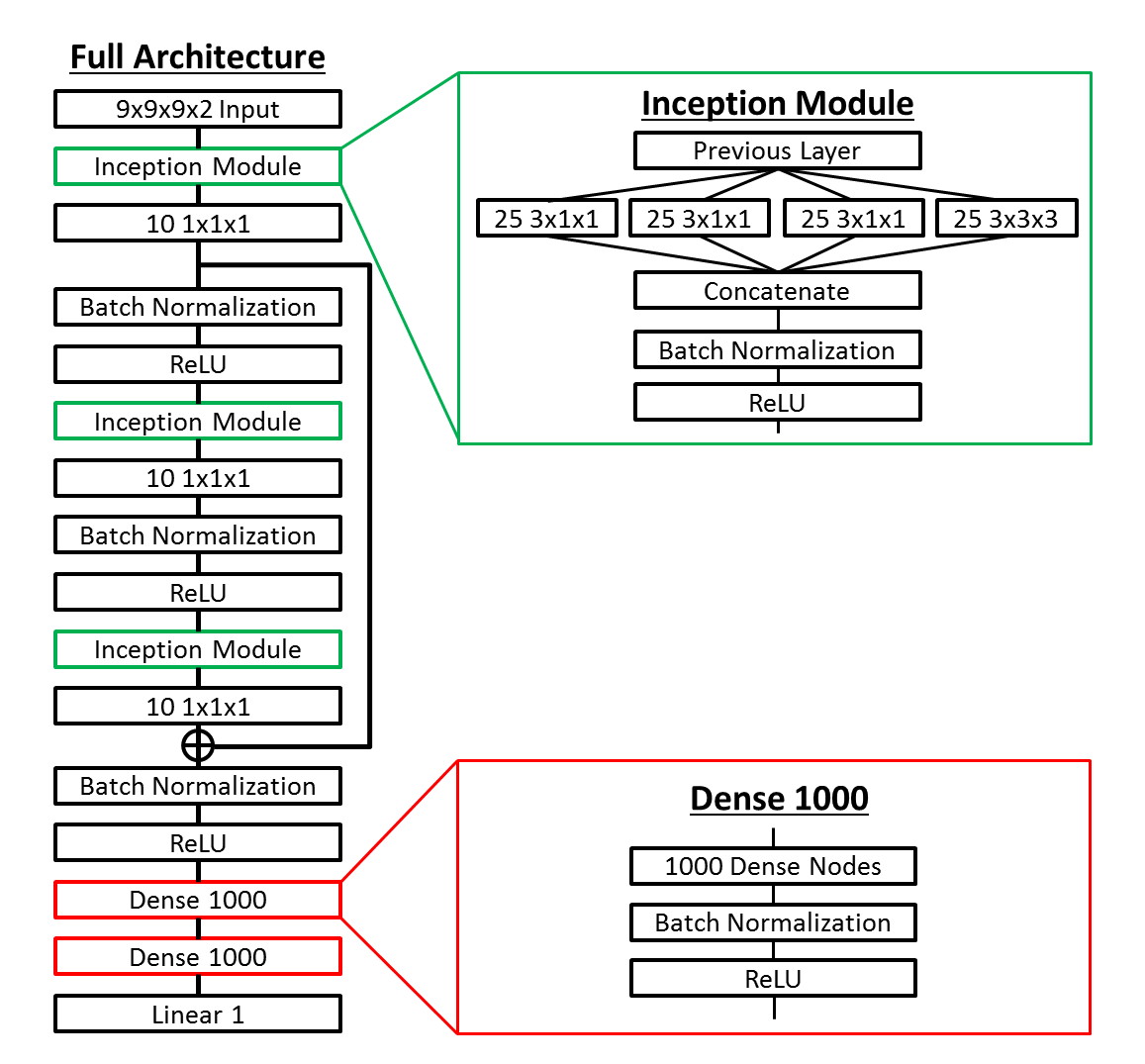
Inhomogeneous Learned Inversion: Simulated datasets were generated using a 3D coupled harmonic oscillators simulation^12,13 as shown in Figure 1. Piecewise smooth input stiffness maps at 2mm isotropic resolution are generated by smoothing 3D Gaussian noise fields with 3D Gaussian kernels of randomly chosen x, y, and z dimensions. The resulting map is scaled such that the maximum and minimum equal randomly selected stiffness values in the range of 0.5 to 15kPa. An ellipsoid inclusion with an independent smoothly varying stiffness profile is inserted in half the simulations to provide sharp stiffness transitions. The damping ratio assigned to each simulation is selected from a uniform distribution of 0 to 0.7. Force drivers are placed at the boundary of the volume and the forward model is solved to generate a wave field. Zero-mean Gaussian noise is added to this wave field, and the real and imaginary components of the temporal first harmonic are used as input features to the ILI neural network (Figure 2). The model was trained on 2.5 million simulated datasets using RMSProp with a batch size of 1000 and a mean squared error (MSE) loss function. Separately generated validation and test sets of 250,000 examples were used in model training and testing. Three decreasing learning rates were used, with training stopped at each learning rate after the MSE failed to improve for three consecutive epochs.

Patient Data: Human data were obtained with institutional review board approval and written informed consent from all patients. Meningiomas allow assessment of the accuracy of ILI in vivo as they have clear borders and their stiffness is known from the surgical report at resection. Limiting our analysis to stiff tumors allows cross-subject analysis of the spatial pattern of stiffness changes. 17 of 64 meningiomas in our MRE database were stiff enough that suction could not remove any part of the tumor and had MRE and T1w data of sufficient quality for inclusion. MRE was acquired at 3mm isotropic resolution at 60Hz as previously described⁶ on clinical 3T scanners (GE Medical Systems, Milwaukee, WI) or a research compact 3T scanner¹⁴. All data was resampled to 2mm isotropic resolution prior to computing the curl and subsequent inversion. The T1w image acquisition and segmentation have been previously described¹⁵. Tumors were manually segmented using the T1w image, with automated segmentation outside of the tumor mask used to define normal brain voxels.

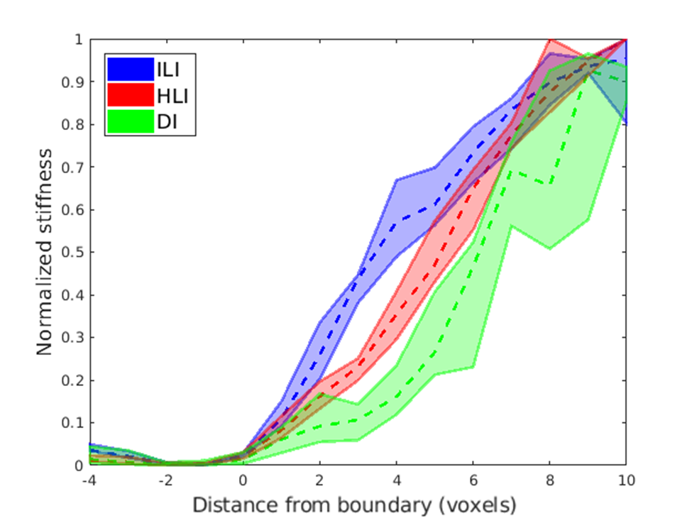
Experiments: ILI is compared to DI and HLI with the same spatial footprint (9x9x9 voxels). Normalized average line profiles across the tumor boundary in all subjects were calculated to evaluate effective inversion resolution. Dice coefficients between the tumor mask and those voxels in the tumor mask exceeding the 95^th percentile of normal brain stiffness are used to assess overall spatial agreement.

Results

Inversion results from DI, HLI, and ILI are shown in a randomly selected case in Figure 3. The ILI inversion results show a sharper transition at the tumor boundary than for HLI or DI (Figure 4). In the Dice coefficient experiment (Figure 5), both HLI and ILI estimated a larger proportion of the tumor as stiffer than the 95^th percentile of normal brain than DI (p<0.0001 for both). There was no significant difference between the Dice coefficients for HLI and ILI.

Discussion and Conclusions

This study offers the first assessment of an inhomogeneous learned inversion in vivo. Incorporating material inhomogeneity into training data allowed ILI to more clearly delineate the margins of meningiomas than inversions assuming material homogeneity with the same footprint. Further, including the full range of physiologic damping ratios and piecewise smooth stiffness variations in training prevented the artefactual stiffness increases seen with an earlier inhomogeneous inversion in vivo. Preliminary results using ILI and HLI with smaller spatial footprints show sharper transition into the tumor than shown here for both inversions. Further exploration of small footprints and addition of non-convex inclusion shapes into training are planned future directions. This study indicates that ILI offers advantages over previously described inversion algorithms for assessment of focal brain lesions.

Acknowledgements

No acknowledgement found.

References

1. Muthupillai, R. et al. Magnetic resonance elastography by direct visualization of propagating acoustic strain waves. Science 269, 1854–1857 (1995).

2. Venkatesh, S. K. et al. MR elastography of liver tumors: preliminary results. AJR Am. J. Roentgenol. 190, 1534–1540 (2008).

3. Shi, Y. et al. Differentiation of benign and malignant solid pancreatic masses using magnetic resonance elastography with spin-echo echo planar imaging and three-dimensional inversion reconstruction: a prospective study. Eur. Radiol. 28, 936–945 (2018).

4. Pepin, K. M. et al. MR Elastography Analysis of Glioma Stiffness and IDH1-Mutation Status. AJNR Am. J. Neuroradiol. 39, 31–36 (2018).

5. Murphy, M. C. et al. Preoperative assessment of meningioma stiffness using magnetic resonance elastography. J. Neurosurg. 118, 643–648 (2013).

6. Hughes, J. D. et al. Higher-Resolution Magnetic Resonance Elastography in Meningiomas to Determine Intratumoral Consistency. Neurosurgery 77, 653–658; discussion 658-659 (2015).

7. Murphy, M. C. et al. Artificial neural networks for stiffness estimation in magnetic resonance elastography. Magn. Reson. Med. 80, 351–360 (2018).

8. Manduca, A. et al. Magnetic resonance elastography: non-invasive mapping of tissue elasticity. Med. Image Anal. 5, 237–254 (2001).

9. McGarry, M. et al. Including spatial information in nonlinear inversion MR elastography using soft prior regularization. IEEE Trans. Med. Imaging 32, 1901–1909 (2013).

10. Scott, J. M. et al. Inhomogeneous Neural Network Inversion (NNI_inh) for stiffness estimation in Magnetic Resonance Elastography. Proc. Intl. Soc. Mag. Reson. Med., Montreal: 2019, 681.

11. Oliphant, T. E., Manduca, A., Ehman, R. L. & Greenleaf, J. F. Complex-valued stiffness reconstruction for magnetic resonance elastography by algebraic inversion of the differential equation. Magn. Reson. Med. 45, 299–310 (2001).

12. Braun, J., Buntkowsky, G., Bernarding, J., Tolxdorff, T. & Sack, I. Simulation and analysis of magnetic resonance elastography wave images using coupled harmonic oscillators and Gaussian local frequency estimation. Magn. Reson. Imaging 19, 703–713 (2001).

13. Sack, I., Bernarding, J. & Braun, J. Analysis of wave patterns in MR elastography of skeletal muscle using coupled harmonic oscillator simulations. Magn. Reson. Imaging 20, 95–104 (2002).

14. Foo, T. K. F. et al. Lightweight, compact, and high-performance 3T MR system for imaging the brain and extremities. Magn. Reson. Med. 80, 2232–2245 (2018).

15. Murphy, M. C. et al. Measuring the characteristic topography of brain stiffness with magnetic resonance elastography. PloS One 8, e81668 (2013).

Figures

Figure 1: ILI is trained on piecewise smooth stiffness maps. An example stiffness map with an ellipsoid inclusion is shown. This stiffness map is the input to a CHO model with 1-10 randomly placed harmonic force drivers with 60Hz frequency. The forward model is solved and a 9x9x9 cube is extracted from the resulting wave simulation. Noise is added to this cube such that the maximum SNR in the cube ranges from 1 to 20. The real and imaginary components of the temporal first harmonic of the noise-added data are the inputs to the neural network.

Figure 2: ILI Neural Network Architecture. The custom convolutional neural network architecture includes three inception modules with a skip connection that lead into two 1000 node dense layers. The output of the network is a stiffness estimate for the center voxel of the cube of wave data it received as input.

Figure 3: ILI clearly delineates boundaries of meningiomas. The T1w image, MRE wave image, and inversion results from DI, HLI, and ILI for a randomly selected case are shown. ILI provides clearer delineation of the tumor margins than DI and HLI.

Figure 4: ILI shows a sharper transition from brain into tumor than HLI and DI with the same spatial footprint. Negative x-axis values represent distance into the brain; positive values into the tumor. Dashed lines are median values; solid lines are 2.5th and 97.5th percentiles (1000 sample bootstrap, case resampling, subjects as cases). To generate this plot, in each subject the median stiffness every distance from the tumor boundary for each inversion was used to generate a line profile, which was scaled from 0 to 1 so that data from all subjects could be combined.

Figure 5: ILI defines more of the tumor as stiffer than normal brain than DI. ILI produces a significantly higher Dice coefficient than DI, suggesting that it better matches the surgeon’s impression at resection that the entire tumor was stiff. Dashed lines connect the individual cases across the inversions. There is no significant difference between HLI and ILI. *p<0.0001, paired one-sided T-test.

Proc. Intl. Soc. Mag. Reson. Med. 28 (2020)

1033