Introduction

$$$T_1$$$-weighted dynamic contrast-enhanced Magnetic Resonance Imaging (DCE-MRI) is typically quantified by least squares (LS) fitting to a pharmacokinetic (PK) model to yield parameters of microvasculature and perfusion in normal and diseased tissues. Such fitting is both time consuming as well as subject to inaccuracy and instability in parameter estimates ¹. Here, we propose a novel neural network approach to estimate the PK parameters by extracting long and short time-dependent features in DCE-MRI.

Methods

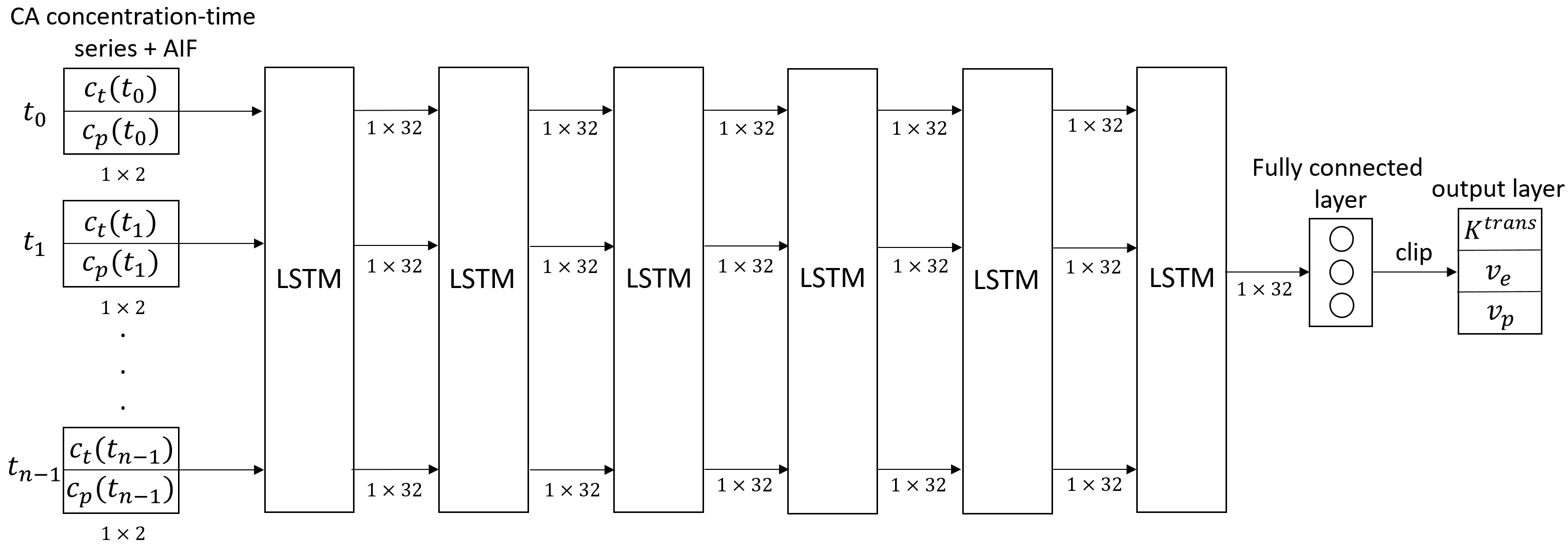
A Long Short-Term Memory (LSTM) network was employed to map DCE-MRI time-series with an arterial input function (AIF) to parameters of the extended Tofts model ².$$C_t(\mathbf{r},t)=K^{trans}(\mathbf{r})\int_0^t C_p(\tau)e^{-\frac{K^{trans}(\mathbf{r})}{v_{e}(\mathbf{r})}(t-\tau)}d\tau+v_p(\mathbf{r})C_p(t)$$ where $$$C_p$$$ and $$$C_t$$$ are the contrast concentration in blood plasma and tissue, respectively, $$$K^{trans}$$$ is the volume transfer rate, $$$v_p$$$ is the fractional plasma volume and $$$v_e$$$ is the fractional interstitial volume. The proposed network (figure 1) consists of 6 LSTM layers with 32 features and a fully connected layer. The network takes an n×2 input that contains the n-dimension signal-time series and the associated AIF. A fully connected layer with 3 features is then applied to generate an estimation of the PK parameters, which are then clipped to a physiologically realistic targeted range, $$$K^{trans} \in [0, 3] (min^{-1})$$$, $$$v_{e} \in [0, 0.4]$$$, and $$$v_{p} \in [0, 0.55]$$$ ^1,3. $$$l_2$$$ loss was used for training.

DCE MR images were acquired from 105 patients with head and neck cancers using a dynamic scanning sequence (TWIST) on a 3 Tesla MRI scanner (Skyra, Siemens Healthineers, Erlangen Germany). Of 105 patients, 80 cases were randomly selected for training, and 25 for testing. For all cases, the subject-specific AIFs were extracted manually ⁴, and the targeted parameter maps were estimated using direct model fitting (DMF) ⁵.

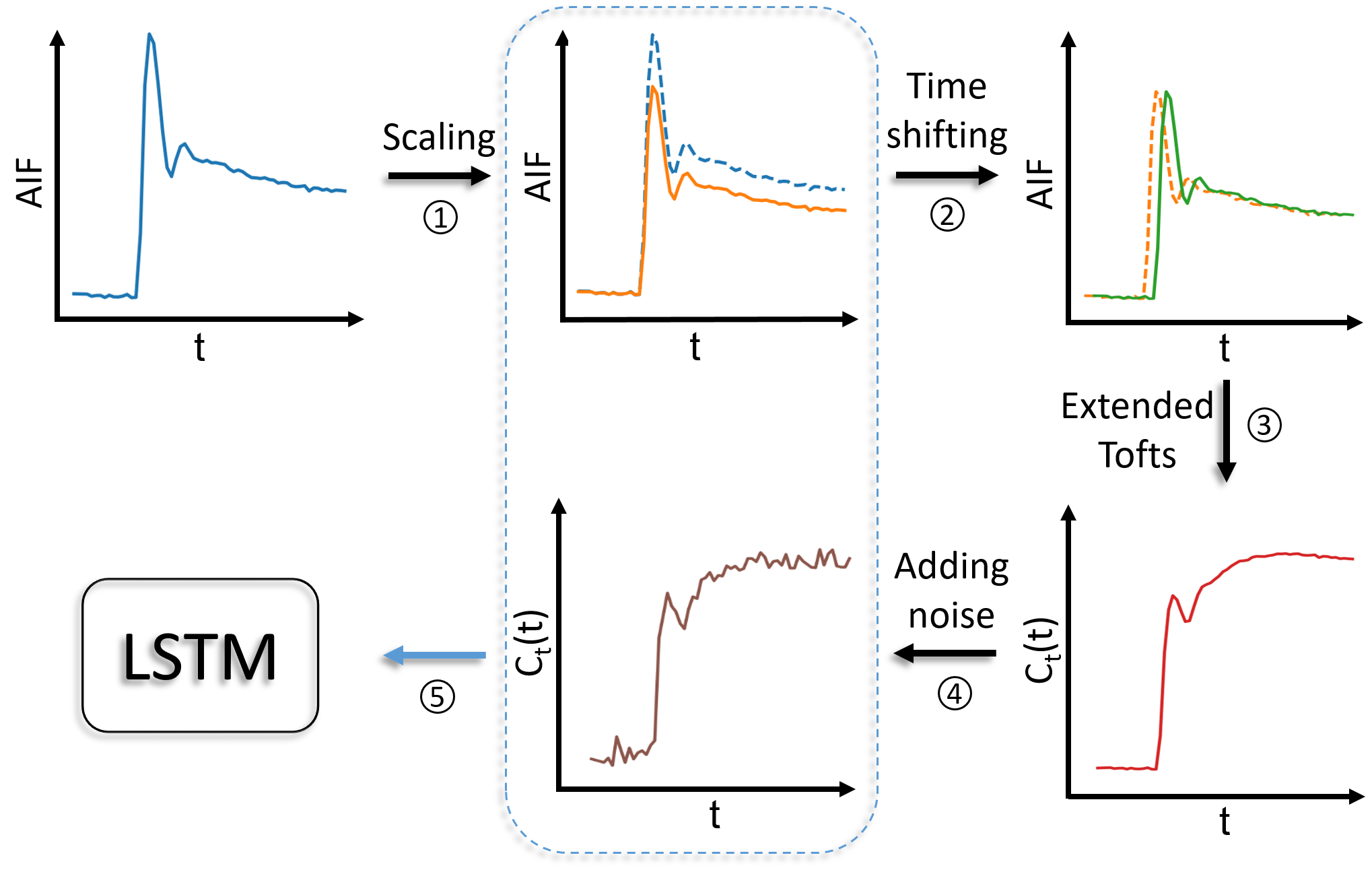
For network training with fully sampled synthetic data, concentration time-curves were generated on-the-fly from randomly drawn AIFs, PK parameters, and time steps ($$$\Delta t$$$) from the training data. Figure 2 shows the data generating process during network training. Random scaling (70%-130%) ⁶ and time-shifting (0-10 seconds to simulate the delay of CA arrival) were applied on each AIF before it was passed into the extended Tofts model, and random Gaussian noise was added to the signal time-series (contrast-to-noise ratio 20-30). The resultant signal time-series and the scaled AIF (without time shifting) were concatenated as an input. The network was trained with Adam optimizer ⁷ with mini-batch size 1000. Two other models with the same architecture as that for the initial model (LSTM3) were trained with 35 cases (LSTM1) and 74 cases (LSTM2) to evaluate the sufficiency of training data. The proposed model was also trained and tested on temporally subsampled synthetic data (by removing intermediate time points) with sampling interval 3s, 4s, 5s, and 6s while maintaining approximately the same total temporal sampling length of 168s..

To evaluate our model, the performance of the LSTM model was compared to both the conventional DMF approach and a CNN model ⁸ trained on 1500 3D volumes with $$$l_2$$$ loss and validated on 300 3D volumes generated using the same dataset as the LSTM training. The performance was quantitatively assessed by the structural similarity (SSIM) index and root mean squared error (rMSE) of the estimated parameter maps with respect to the ground truth parameter maps.

Results

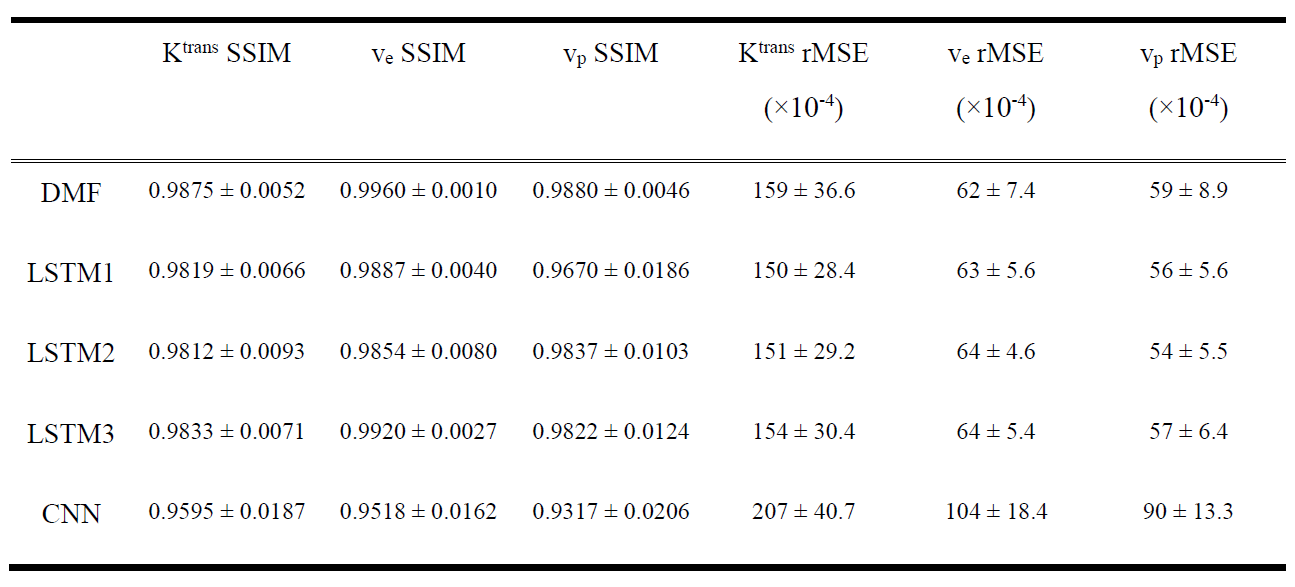
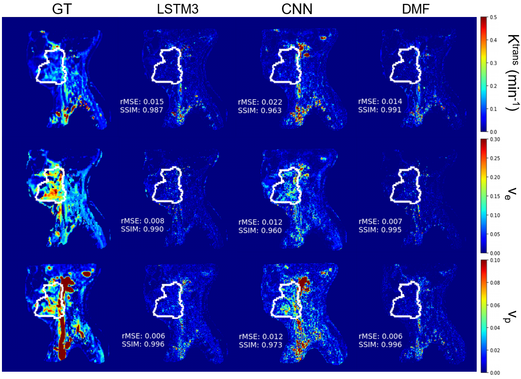
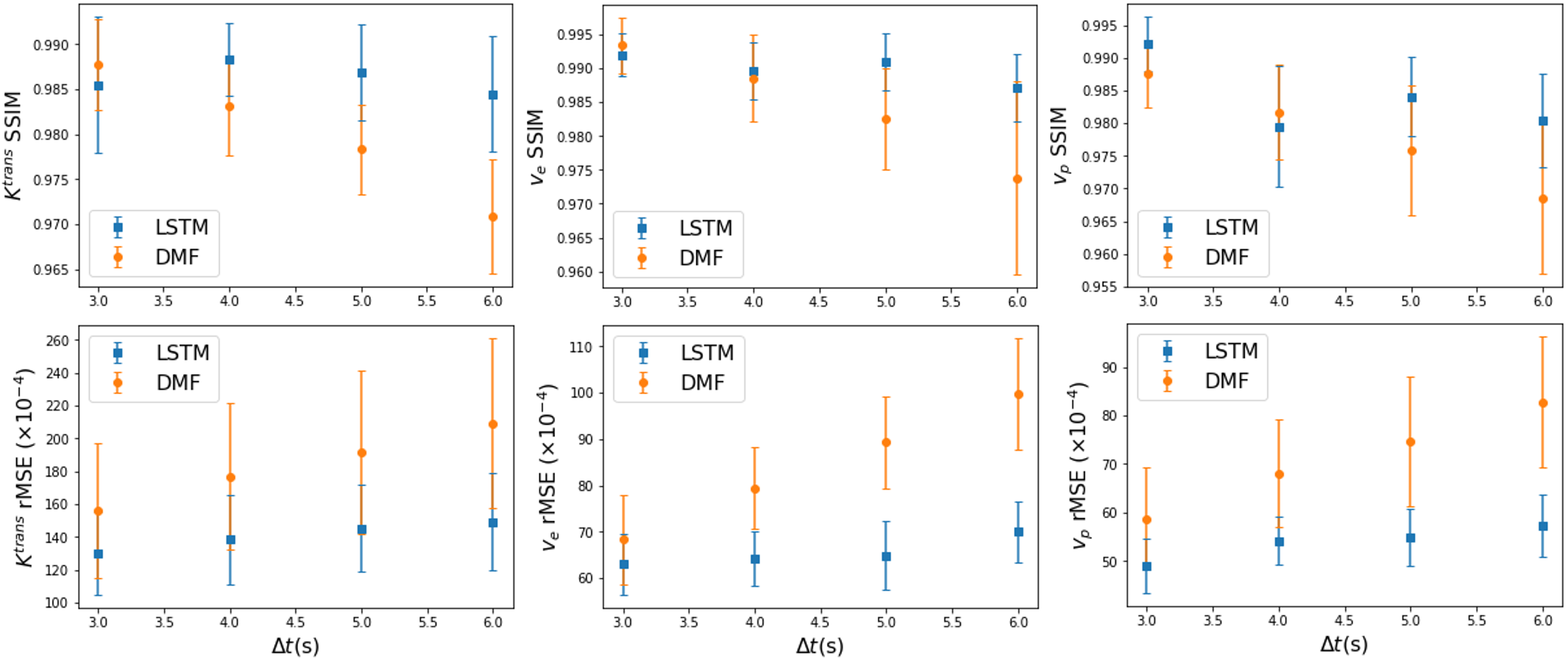
The performance of the LSTM network on fully temporal sampled synthetic signals were compared to the CNN and DMF models (table 1). The LSTM3 had similar performance but 90 folds of computation time reduction compared to the DMF approach (table 1). The LSTM3 outperformed the CNN-based approach by reducing the rMSE up to 62%. The performance of LSTM1, LSTM2 and LSTM3 were similar, indicating the training data augmentation was effective. Figure 3 shows the PK parameter estimation residual maps of an exemplary slice of the testing data by different methods.

For temporally subsampled simulated signals, the LSTM method consistently outperformed the DMF approach when the sampling time interval of the dynamic signals is 4s or greater (figure 4). While the average rMSE and SSIM from the DMF degraded significantly with an increase in the sampling interval, the LSTM approach showed a robust performance for sparse temporal sampling data.

Discussion and conclusion

The superior performance of the LSTM to a CNN-based approach is attributed to the capability of LSTM to learn long- and short-term dependency of sequence data in the DCE-MRI. Also, the LSTM model was more robust to temporally sparsely sampled DCE data than the DMF, which allows to increase spatial resolution of DCE images. Our data augmentation strategies, including AIF augmentation on-the-fly, overcame the limited size of the in vivo DCE-MRI data. The LSTM network trained by synthesized data was also able to perform well on empirical DCE data. This is likely due to that the synthetic data simulates real signal intensity-time series well and the network is effectively trained. In addition, our proposed network enables an approximately 90× computation time acceleration compared with the DMF approach. The LSTM network has the potential to accelerate DCE-MRI acquisition and parameter estimation.

Acknowledgements

This work was supported by NIH R01 EB016079.