1029
Exploration of Feature Space in Semantic Segmentation Convolutional Neural Networks1Electrical Engineering, Brigham Young University, Provo, UT, United States, 2Electrical Engineering, Stanford University, Stanford, CA, United States, 3Radiology, Stanford University, Stanford, CA, United States, 4Bioengineering, Stanford University, Stanford, CA, United States, 5Orthopedic Surgery, Stanford University, Stanford, CA, United States, 6Bioengineering, Imperial College London, London, United Kingdom
Synopsis
Recent advances in deep learning and convolutional neural networks (CNNs) have shown promise for automatic segmentation in MR images. However, because of the stochastic nature of the training process, it is difficult to interpret what information networks learn to represent. In this study, we explore how differences in learned weights between networks can be used to express semantic relationships between different tissues. For cartilage and meniscus segmentation in the knee, we show that network generalizability for segmenting tissues can be measured by distances between networks. We also use these findings to motivate robust training policies for fine-tuning with limited data.
Introduction
In recent years, convolutional neural networks (CNNs) have shown potential for rapid, high-fidelity automatic segmentation of MR images. However, because of their stochastic nature, it is difficult to characterize network behavior and interpret how networks represent relevant information. Recent work has explored how different learning environments influence overall segmentation performance1,2, but has not characterized how these networks learn relationships between different tissues. A deeper analysis into the learned representations (“features”) of different tissues may allow for improved interpretation of how networks leverage spatial proximity among tissues. In this study, we performed segmentation of femoral cartilage, tibial cartilage and menisci as an archetype of segmenting tissues in the knee of varying volumes. By comparing the distance between trained weights of nine different segmentation neural networks, we quantified the distance between tissue spatial features as a metric for characterizing semantic relationships between tissues.Methods
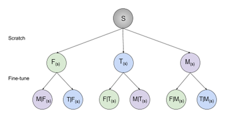
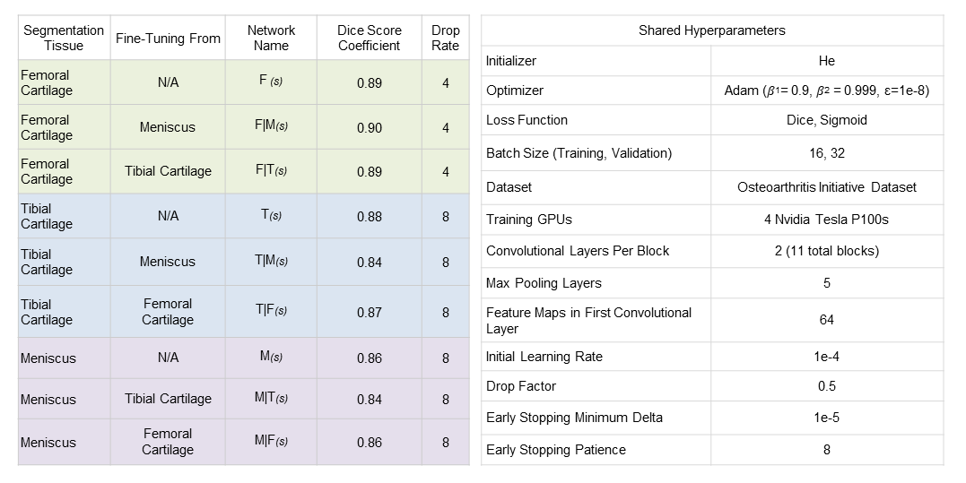
The state-of-the-art 2D U-Net architecture3 was used to train nine single-class segmentation models on 3D double-echo steady-state volumes acquired from the Osteoarthritis Initiative4. 88 subjects scanned at two timepoints were randomly split into cohorts of 60 (120), 14 (28), 14 (28) subjects (scans) for training, validation, and testing, respectively.Three separate networks were trained to segment femoral cartilage, tibial cartilage, and menisci (termed “scratch” networks) from convolutional weights randomly initialized using He initialization5. Each “scratch” network was subsequently fine-tuned to segment the remaining two tissues independently, resulting in a total of 9 networks, 3 (1 scratch, 2 fine-tuned) for each tissue (Fig. 1). The following convention is introduced: A(s)-network trained to segment tissue A from scratch, B|A(s)-network to segment tissue B by fine-tuning on weights of A(s).
Training hyperparameters were empirically chosen to maximize network performance (Fig. 2). Early stopping was used during training to avoid overfitting6. Network weights resulting in the lowest soft-Dice validation loss were used for comparison.
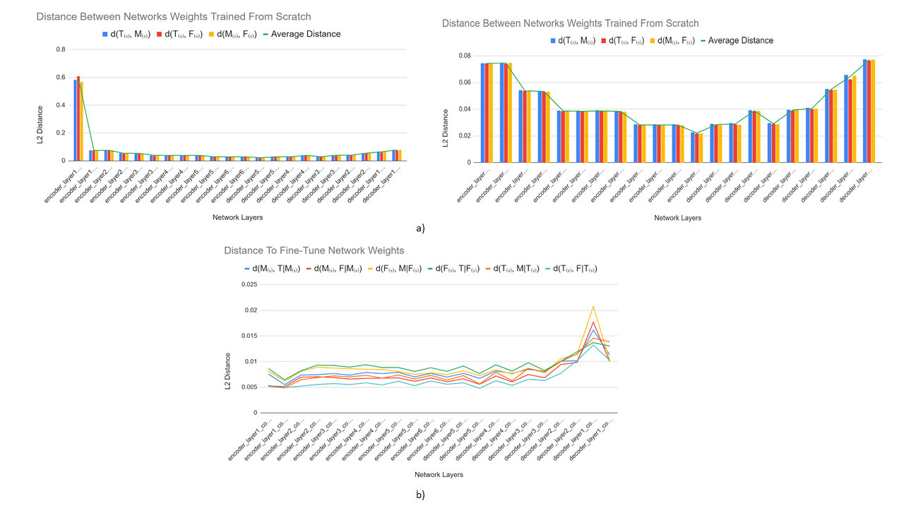
To better understand how networks learn to segment a new class from initial training, we observe the extent to which networks weights evolve during fine-tuning. The average Euclidean (L2) distance ‘d’ between learned convolution kernel weights of two networks was used to quantify network similarity. Distances were computed across the entire network and for corresponding weights at different depths of the U-Net architecture. The average feature distances between two tissues A,B were calculated as averages of bidirectional distances d(A(s),B|A(s)) and d(B(s),A|B(s)). Activation maps were generated to visualize similarities in activation regions among different networks.
Results
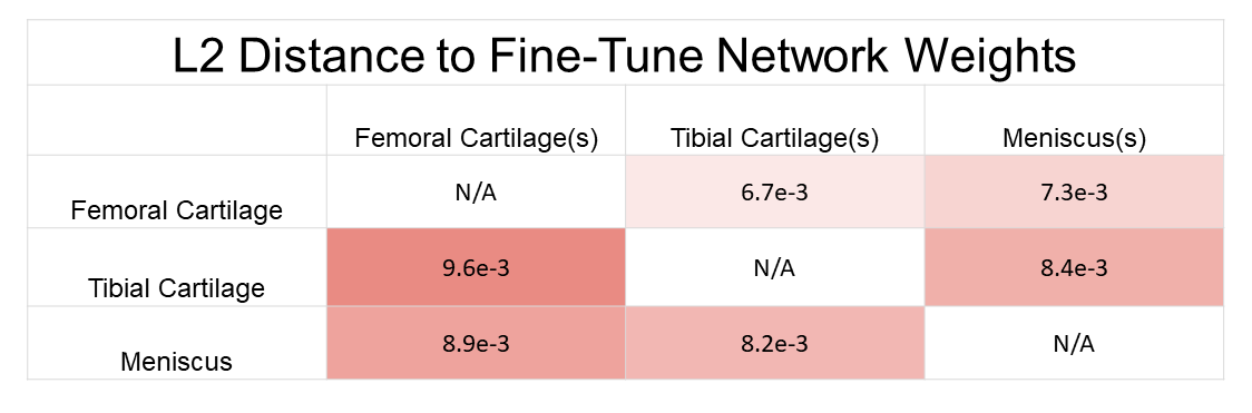
Longer distances between scratch networks were observed at shallower regions of the network, while latent layers (enc_layer6) had the least difference (Fig. 3a). Distances between scratch networks and their corresponding fine-tuned networks were longest in shallower decoder stages (dec_layer1) (Fig. 3b). On average, networks fine-tuned to segment a particular tissue had a shorter distance to their base scratch networks (d=8.17e-3) than to other scratch networks trained to segment the same tissue (d=6.45e-2).Average distances between tissues were 8.13e-3 between femoral cartilage and tibial cartilage, 8.07e-3 between femoral cartilage and meniscus, and 8.32e-3 between meniscus and tibial cartilage. Bidirectional distances between femoral cartilage and tibial cartilage were asymmetric: d(F,T|F(s))=9.56e-3, d(T(s),F|T(s))=6.70e-3. However, bidirectional distances between meniscus and femoral cartilage and meniscus and tibial cartilage were more symmetric (Fig. 4).
Additionally, networks fine-tuned to segment tibial cartilage and meniscus performed worse than their from-scratch counterparts (Fig. 2).
Discussion
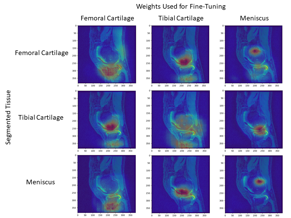
Shorter, near-equal distances in the latent space among scratch networks may suggest that high-level representations for a single tissue are shared amongst latent representations of other tissues of interest.Furthermore, fine-tuned networks segmenting femoral cartilage performed more similarly to their from-scratch counterpart compared to those segmenting tibial cartilage or meniscus (Fig. 2). Networks segmenting femoral cartilage also shared activation regions with both tibial cartilage and meniscus segmentation networks (Fig. 5). This may suggest that latent representations of femoral cartilage are conditioned on more representative of features of the whole image.
The asymmetry in bidirectional network distances may also quantify the extent to which certain tissue representations are generalizable to other tissues. The asymmetry between femoral cartilage and tibial cartilage and the minimal difference in performance among femoral cartilage segmentation networks may suggest that femoral cartilage has a larger spatial span of optimal feature representations compared to tibial cartilage. This may facilitate fine-tuning networks trained on other tissues to segment femoral cartilage.
Similarities in tissue features may enable shaping training policies in cases of limited data. Tissue pairs with shorter, symmetric distances may be better suited for fine-tuning on the other tissue. Additionally, limited changes in latent embeddings between these tissues can allow depth-dependent learning rates, where deeper, latent features change slower compared to shallower representations. This may reduce the amount of training data required for network convergence while maximizing performance on segmenting the new tissue. Moreover, tissues with a larger set of optimal feature representations, such as femoral cartilage, may require less data when fine-tuned on networks trained on other tissues.
Conclusion
We characterize semantic relationships between tissues by inspecting learned feature representations for tissue segmentation. We show that the distance between feature weights can be used to interpret similarity in latent features between tissues and to design training policies for network fine-tuning without compromising performance.Acknowledgements
NIH R01-EB002524-14, NIH K24-AR062068-07, NIH R01-AR063643-05, NSF 1656518, Stanford Medicine Precision Health and Integrated Diagnostics, GE Healthcare, PhilipsReferences
1. Garcia-Garcia, et al. “A Review on Deep Learning Techniques Applied to Semantic Segmentation”, Submitted to TPAMI, April 2017
2. Desai, et al. “Technical Considerations for Semantic Segmentation in MRI using Convolutional Neural Networks”, Submitted to Magnetic Resonance in Medicine. Accessed 2019.
3. Ronneberger, et al. “U-Net: Convolutional Networks for Biomedical Image Segmentation”, MICCAI 2015:234-241
4. Peterfy, et al. “The osteoarthritis initiative: report on the design rationale for the magnetic resonance imaging protocol for the knee”, Osteoarthritis and Cartilage. 2008:16(12);1433-1441.
5. He et al. “Delving Deep into Rectifiers: Surpassing Human-Level Performance on ImageNet Classification”, International Conference on Computer Vision (ICCV), 2015.
6. Prechelt, Lutz. “Early Stopping - But When?”, Neural Networks: Tricks of the Trade. 1998:1524;55-69.
Figures