1020

Myelin Water Imaging Using STFR with Exchange

Steven T. Whitaker¹, Gopal Nataraj², Jon-Fredrik Nielsen³, and Jeffrey A. Fessler¹
¹Electrical Engineering and Computer Science, University of Michigan, Ann Arbor, MI, United States, ²Medical Physics, Memorial Sloan Kettering Cancer Center, New York, NY, United States, ³Biomedical Engineering, University of Michigan, Ann Arbor, MI, United States

Synopsis

Myelin water fraction (MWF) estimates are desirable for tracking the progression of demyelinating diseases such as multiple sclerosis. To address the long scan times of conventional MWF imaging methods, faster steady-state scans have been studied recently. One such steady-state scan is small-tip fast recovery (STFR). This work compares STFR-based MWF estimates using a two-compartment tissue model without exchange to those obtained using a three-compartment tissue model with exchange. Using a three-compartment model with exchange results in MWF estimates that are closer to traditional multi-echo spin echo (MESE) estimates.

Introduction

Myelin water fraction (MWF) estimates are desirable for tracking the progression of demyelinating diseases such as multiple sclerosis. A common way to estimate MWF is from multi-echo spin echo (MESE) scans.¹ Work has been done to speed up MESE acquisitions ², but they are still speed-limited by a long TR requirement. As a result, faster steady-state scans have been studied ^3-9, including small-tip fast recovery (STFR).¹⁰ A recent MWF estimation method used STFR scans optimized for precision.¹¹ That work assumed each voxel consisted of two compartments, myelin water and non-myelin water, and that the two compartments did not exchange with each other. However, neglecting exchange leads to biases in MWF estimates.¹² Here, we use a three-compartment tissue model: myelin water, non-myelin water, and a macromolecular pool; myelin water and non-myelin water are in exchange, while myelin water exchanges with the macromolecular pool.¹³ We compare MWF estimates derived from STFR scans using the two-compartment model without exchange to those derived using the three-compartment model with exchange. We also compare the STFR-based MWF estimates to MESE-based estimates.

Methods

For a two-compartment tissue model without exchange, the Bloch-McConnell equation solution ¹⁴ reduces to the weighted sum of two single-compartment signals, where the weights for the myelin and non-myelin water compartments are MWF and 1-MWF, respectively. STFR has an analytical signal model for the single compartment case ¹⁰, so the two-compartment STFR signal model is computationally efficient. With exchange, the Bloch-McConnell equation lacks an analytical solution, which makes computing the STFR signal from the three-compartment model more challenging. Figure 1 illustrates the differences between the two tissue models.
We first compared the two tissue models in simulation. We simulated STFR and MESE scans for typical white matter and gray matter tissue parameters using the three-compartment model with exchange. These simulations were computed by numerically solving the Bloch-McConnell equation. For the STFR scans, we used scan parameters that were optimized to minimize the Cramer-Rao Lower Bound (CRLB) of unbiased estimates of MWF ¹⁵, as done in ¹¹. For the MESE scan, we used a 90° excitation followed by 32 refocusing (180°) pulses. The echo spacing was 10 ms, and the repetition time was 1200 ms.
After simulating the scans, we estimated MWF from the STFR scans using a kernel-based estimation method (PERK).¹⁶ In one case, we generated noisy simulated data using the two-compartment model without exchange to train PERK and then estimated MWF. We compared these MWF estimates to those given by PERK when trained on data simulated using the three-compartment model with exchange. We compared these STFR-based MWF estimates to MESE-based estimates, which were obtained using regularized non-negative least squares (NNLS), following the approach in ¹⁷.
We next compared the two tissue models in vivo. We acquired STFR and MESE scans of a healthy volunteer using the same scan parameters as in simulation. We also acquired a pair of Bloch-Siegert (BS) scans for separate B1+ estimation (used in the STFR-based MWF estimation). The scans were 3D acquisitions with matrix size 200 $$$\times$$$ 200 $$$\times$$$ 9 and isotropic 1.1 mm resolution. The STFR and BS scans combined took 7 min 14 s, and the MESE scan took 36 min 11 s. As in simulation, we estimated MWF from the STFR scans using PERK; in one case PERK was trained using the two-compartment model without exchange, and in the other case PERK was trained using the three-compartment model with exchange. We also estimated MWF from the MESE data using NNLS.

Results

Figure 2 and Table 1 summarize simulation results. The STFR-based MWF estimates when training PERK using the two-compartment tissue model without exchange are highly overestimated, whereas those obtained using the three-compartment model with exchange are much closer to the true MWF. The MESE-based MWF estimates are underestimated, likely because NNLS does not account for exchange.
Figure 3 and Table 2 summarize in vivo results. Again, the STFR-based MWF estimates when training with the two-compartment model are higher than those obtained when training with the three-compartment model. These latter estimates are closer to the MESE-based MWF estimates. The MESE MWF map appears noisier than those shown in other works, which is likely due to the lower SNR of our data due to differences in voxel size. To match the STFR resolution, we acquired MESE with 1.1 mm isotropic voxels, whereas often MESE data is collected with slice thickness of 5 mm and 1.6 mm or greater in the phase encode direction.

Discussion

We estimated MWF from STFR scans using PERK. We compared estimates when training with a two-compartment non-exchanging model to those obtained when training with a three-compartment exchanging model. Training with the three-compartment model led to more accurate MWF estimates in simulation and in vivo estimates that were closer to MESE-based MWF estimates.
We focused on a three-compartment tissue model in this work, where we combined intra- and extra-cellular water pools into a single, non-myelin water compartment. One could separate these into two compartments, resulting in a four-compartment model. Further work is needed to determine whether the additional model complexity leads to significantly better MWF estimates.

Acknowledgements

We thank Dr. Navid Seraji-Bozorgzad for discussions of in vivo results.

This work was supported by NIH R21 AG061839.

References

[1] A. Mackay, K. Whittall, J. Adler, D. Li, D. Paty, and D. Graeb. In vivo visualization of myelin water in brain by magnetic resonance. Mag. Res. Med., 31(6):673-7, June 1994.

[2] T. Prasloski, A. Rauscher, A. L. MacKay, M. Hodgson, I. M. Vavasour, C. Laule, and B. Madler. Rapid whole cerebrum myelin water imaging using a 3D GRASE sequence. NeuroImage, 63(1):533-9, October 2012.

[3] G. Nataraj, J-F. Nielsen, and J. A. Fessler. Myelin water fraction estimation from optimized steady-state sequences using kernel ridge regression. In Proc. Intl. Soc. Mag. Res. Med., page 5076, 2017.

[4] G. Nataraj, M. Gao, J-F. Nielsen, and J. A. Fessler. Kernel regression for fast myelin water imaging. In ISMRM Workshop on Machine Learning Part 2, page 65, 2018.

[5] G. Nataraj, J-F. Nielsen, M. Gao, and J. A. Fessler. Fast, precise myelin water quantification using DESS MRI and kernel learning. Technical report, 2018. http://arxiv.org/abs/1809.08908.

[6] D. Hwang, D-H. Kim, and Y. P. Du. In vivo multi-slice mapping of myelin water content using T2* decay. NeuroImage, 52(1):198-204, August 2010.

[7] C. Lenz, M. Klarhofer, and K. Scheffler. Feasibility of in vivo myelin water imaging using 3d multigradient-echo pulse sequences. Mag. Res. Med., 68(2):523-8, August 2012.

[8] S. C. L. Deoni, B. K. Rutt, T. Arun, C. Pierpaoli, and D. K. Jones. Gleaning multicomponent T1 and T2 information from steady-state imaging data. Mag. Res. Med., 60(6):1372-87, December 2008.

[9] S. T. Whitaker, G. Nataraj, J-F. Nielsen, and J. A. Fessler. Myelin water fraction estimation using small-tip fast recovery MRI. Mag. Res. Med., Submitted 2019.

[10] J-F. Nielsen, D. Yoon, and D. C. Noll. Small-tip fast recovery imaging using non-slice-selective tailored tip-up pulses and radiofrequency-spoiling. Mag. Res. Med., 69(3):657-66, March 2013.

[11] S. T. Whitaker, G. Nataraj, M. Gao, J-F. Nielsen, and J. A. Fessler. Myelin water fraction estimation using small-tip fast recovery MRI. In Proc. Intl. Soc. Mag. Res. Med., page 4403, 2019.

[12] K. D. Harkins, A. N. Dula, and M. D. Does. Effect of intercompartmental water exchange on the apparent myelin water fraction in multiexponential T2 measurements of rat spinal cord. Mag. Res.Med., 67(3):793-800, March 2012.

[13] G. J. Stanisz, A. Kecojevic, M. J. Bronskill, and R. M. Henkelman. Characterizing white matter with magnetization transfer and T2. Mag. Res. Med., 42(6):1128-36, December 1999.

[14] H. M. McConnell. Reaction rates by nuclear magnetic resonance. J. of Chemical Phys., 28(3):430-31,March 1958.

[15] G. Nataraj, J-F. Nielsen, and J. A. Fessler. Optimizing MR scan design for model-based T1, T2 estimation from steady-state sequences. IEEE Trans. Med. Imag., 36(2):467-77, February 2017.

[16] G. Nataraj, J-F. Nielsen, C. D. Scott, and J. A. Fessler. Dictionary-free MRI PERK: Parameter estimation via regression with kernels. IEEE Trans. Med. Imag., 37(9):2103-14, September 2018.

[17] T. Prasloski, B. Madler, Q-S. Xiang, A. MacKay, and C. Jones. Applications of stimulated echo correction to multicomponent T2 analysis. Mag. Res. Med., 67(6):1803-14, June 2012.

[18] K. L. Miller, S. M. Smith, and P. Jezzard. Asymmetries of the balanced SSFP profile. Part II: White matter. Mag. Res. Med., 63(2):396-406, February 2010.

[19] D. L. Collins, A. P. Zijdenbos, V. Kollokian, J. G. Sled, N. J. Kabani, C. J. Holmes, and A. C. Evans. Design and construction of a realistic digital brain phantom. IEEE Trans. Med. Imag., 17(3):463-8,June 1998.

Figures

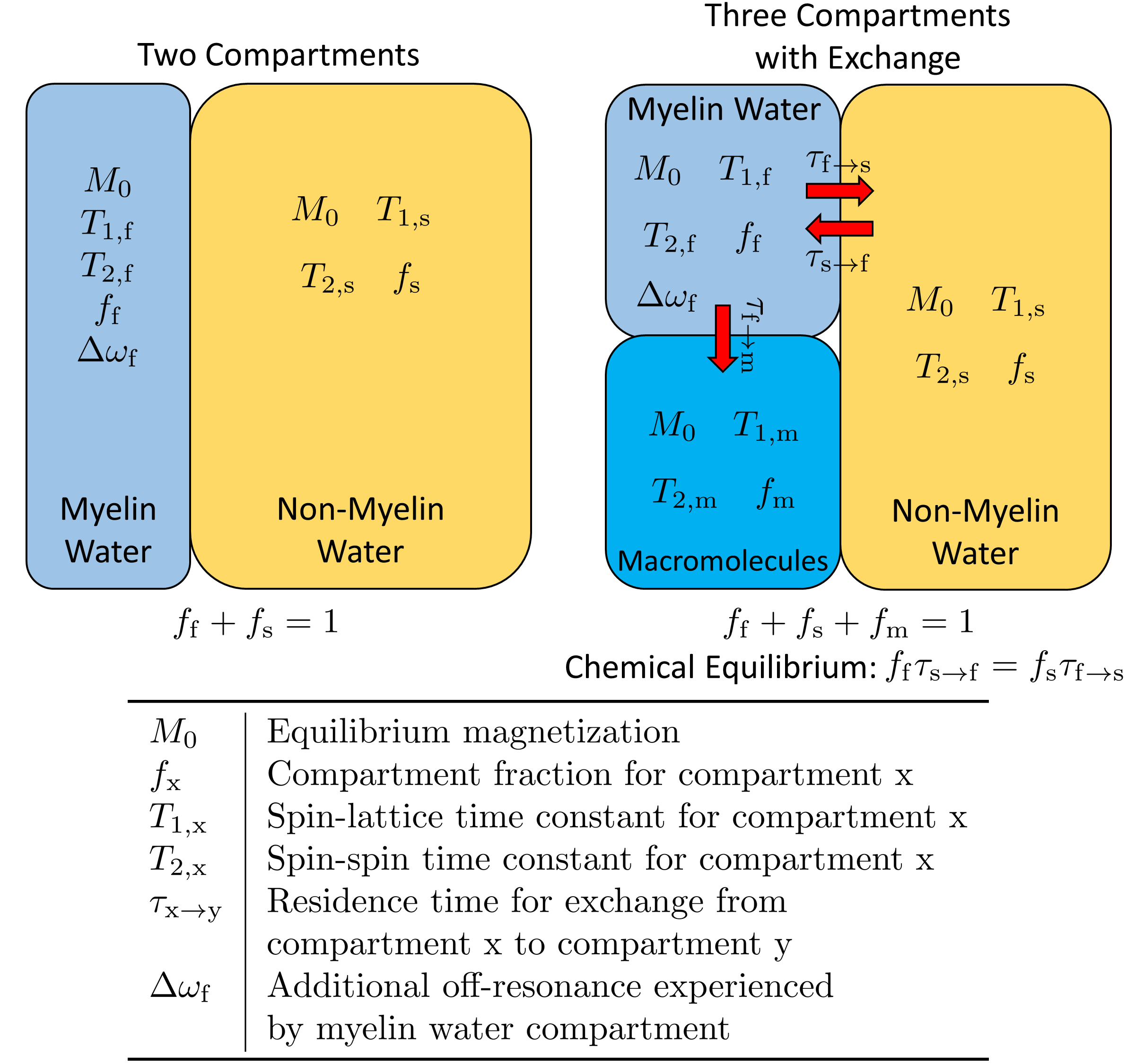
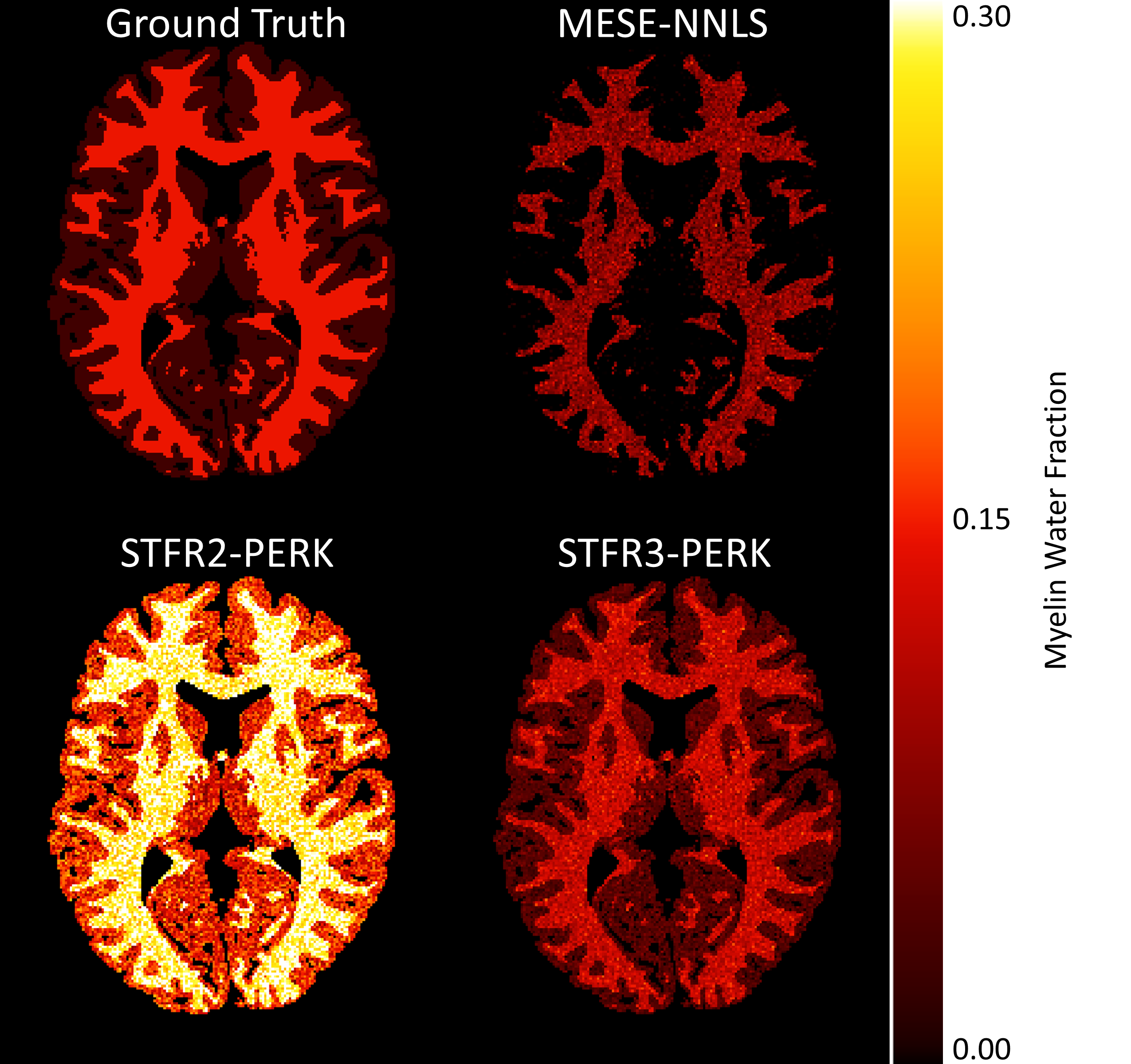
Figure 1: Illustration of the two-compartment and three-compartment tissue models. The subscripts "f", "s", and "m" represent, respectively, myelin water, non-myelin water, and macromolecules. In both cases, we model the additional off-resonance experienced by the myelin water compartment.¹⁸ Other myelin water imaging works typically ignore this additional off-resonance parameter.

Figure 2: MWF maps from simulated test data for a three-compartment tissue model with exchange. STFR2-PERK shows MWF estimation using PERK trained with the two-compartment non-exchanging STFR model. STFR3-PERK shows MWF estimation using PERK trained with the three-compartment exchanging STFR model. MESE-NNLS shows MWF estimation using MESE and regularized NNLS. Using the three-compartment model results in more accurate MWF estimates than the two-compartment model. Table 2 reports numerical results. The anatomy for this simulated data is from BrainWeb.¹⁹

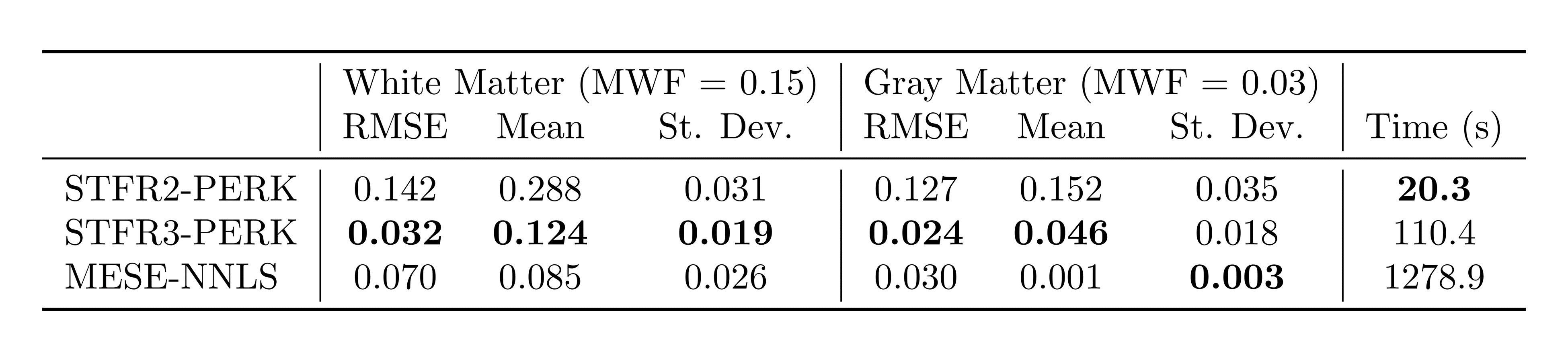
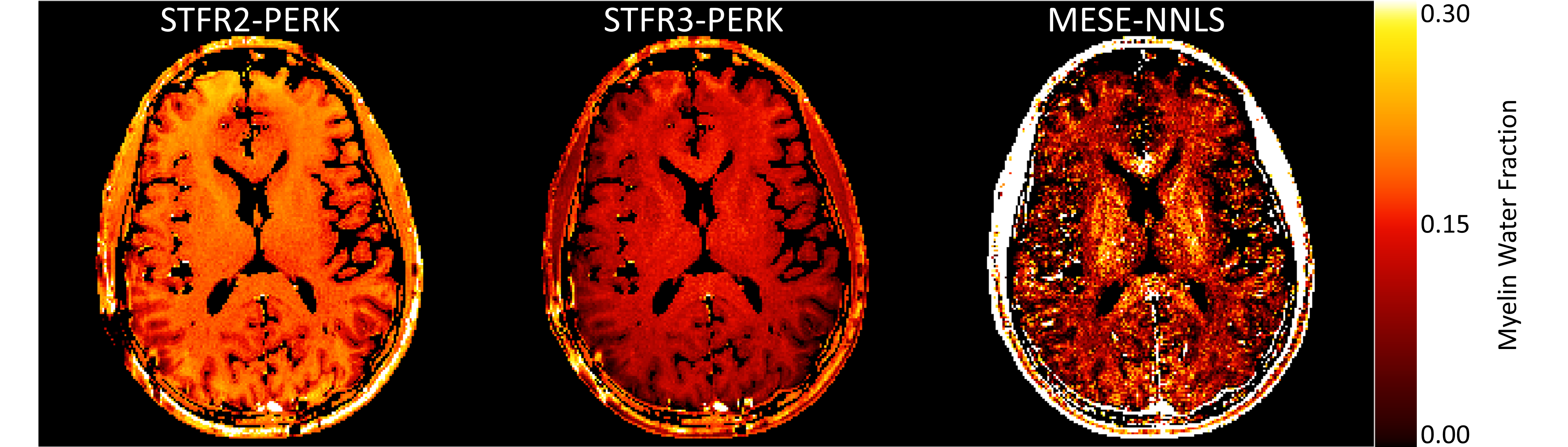
Table 1: Numerical results associated with Figure 1. The reported time refers to the entire estimation, combining the time to estimate MWF in white matter voxels and gray matter voxels; it also includes training time for the methods that use PERK. The best value in each column is highlighted. Using the three-compartment model results in more accurate MWF estimates than using the two-compartment model. Furthermore, STFR3-PERK is the most accurate of the three methods compared here.

Figure 3: MWF maps from in vivo MESE data and STFR data. STFR2-PERK shows MWF estimation using PERK with the two-compartment non-exchanging STFR model. STFR3-PERK shows MWF estimation using PERK with the three-compartment exchanging STFR model. MESE-NNLS shows MWF estimation using MESE and regularized NNLS. Using the three-compartment model results in MWF estimates that are closer to MESE-NNLS values than using the two-compartment model. Table 3 shows numerical results for several manually selected regions of interest.

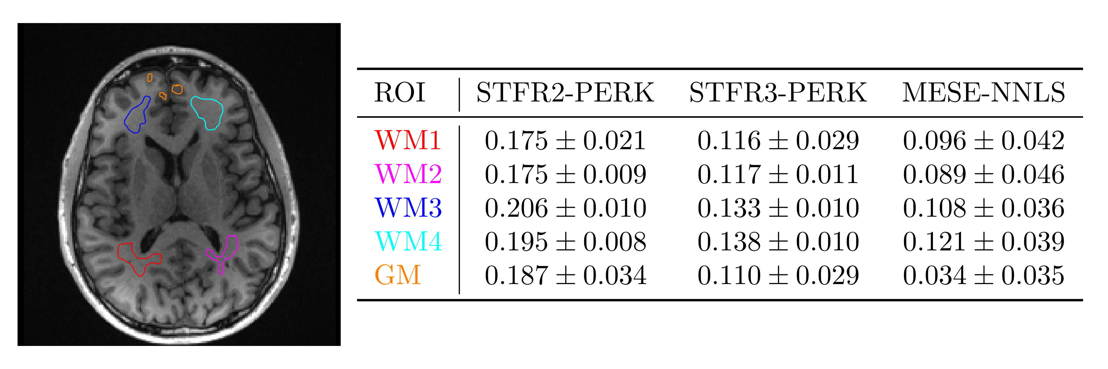
Table 2: Left: White matter (WM) and gray matter (GM) regions of interest (ROIs). The underlying image is from a standard MP-RAGE acquisition, acquired in the same scan session and registered to the other scans. Right: Sample means $$$\pm$$$ standard deviations of MWF estimates for four WM ROIs and one GM ROI for the MWF maps in Figure 3. The two-compartment STFR2-PERK MWF estimates differ significantly from the MESE-NNLS estimates,whereas,for each WM ROI,the STFR3-PERK MWF estimates match the MESE-NNLS estimates to within one standard deviation.

Proc. Intl. Soc. Mag. Reson. Med. 28 (2020)

1020