Introduction

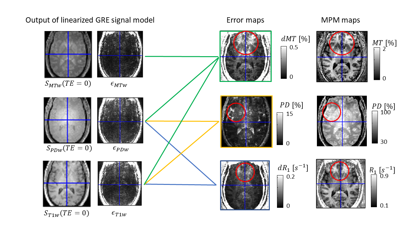
In contrast to standard weighted images, Multi-Parameter Mapping (MPM)^1,2 provides multiple quantitative markers (longitudinal relaxation rate R₁, proton density PD, effective transverse relaxation rate R₂^*, and magnetization transfer saturation MT). These parameter maps are more specific to key biological features, e.g. myelin and iron content³. However, since requiring the combination of multiple multi-echo fast-low-angle-shot (FLASH⁶) volumes, MPMs are also more susceptible to subject motion than traditional morphometric features such as volumetry from weighted images. In addition, the parameter estimation is based on the nonlinear relation between acquired signal and quantitative model parameters, which can amplify errors in the underlying FLASH data, e.g. caused by subject motion or physiological noise.
In this study, we introduce a method to calculate error maps that are sensitive to erroneous regions in the quantiatiave MPM maps (Fig.1). For correction of errors, we introduce a method to calculate a weighted average over repeated MPMs using voxel-based weights reflecting local parameter error.

Methods

Subjects: We included 10 healthy participants in the reported analysis (M_age=31.3 years, 7 female). Exclusion criteria were psychiatric disorders, assessed via the Mini-International Neuropsychiatric Interview⁴, neurological diseases, head trauma or metallic implants.
MRI: Scans were performed on a 3T PRISMA MRI (Siemens Healthcare, Erlangen, Germany), using the Siemens 64-channel receiver (Rx) head-coil. Whole brain MR images were acquired using the MPM² protocol, including calibration⁵ and three different weightings (MT-, PD- and T₁-weighting) FLASH images. The following sequence parameters were used: isotropic resolution of (1 mm)³, flip angle (FA) of 6° (for MT- and PD-weighted) and 21° (for T₁-weighted), 8 echoes (2.30 to 18.40 ms, in steps of 2.30 ms), readout bandwidth of 488 Hz/pixel, and repetition time (TR) of 24.00 ms. The weighted images were acquired in two successive runs using a 3D acceleration factor of 3 and partial Fourier (6/8) (28 min.).
Step 1: Estimation of the model-fit residuals $$$\vec{\epsilon}_{inx}$$$ for each gradient-recall echo signal with PD-, T₁-, and MT-weighting ($$$inx \in \{ PDw, T1w, MTw \}$$$) using the linearized exponential signal decay : $$ (1) \vec{y}_{inx}=\vec{\underline{X}\beta}_{inx}+\vec{\epsilon}_{inx}$$ with $$$\vec{y}=\ln\begin{pmatrix}S_{inx}(TE_1) \\ \vdots \\ S_{inx}(TE_N)\end{pmatrix}$$$, $$$\underline{X}$$$ being an $$$N \times 2$$$ matrix with rows $$$X_k = \left[ 1, TE_k \right], k\in 1,\dots,N$$$ where $$$N$$$ is the number of echoes and $$$\vec{\beta}_{inx}$$$ are regression coefficients. The root-mean-square of the model-fit residuals $$$\left(\epsilon_{inx} = rms\left(\vec{\epsilon}_{inx}\right)\right)$$$ was used in the next steps.
Step 2: To estimate the error of each quantitative map (Fig.1), we calculated the propagation of error for uncorrelated errors (for a function $$$F(x,y)$$$, it is defined as follows: $$$dF(x,y)=\sqrt{\left(\frac{dF}{dx}\right)^2 dx^2+\left(\frac{dF}{dy}\right)^2dy^2}$$$ ). For example, the error for the example of R₁ was defined as follows: $$ (2) dR_1=\sqrt{\left(\frac{dR_1}{dS_{T1w}}\epsilon_{T1w}\right)^2+\left(\frac{dR_1}{dS_{PDw}}\epsilon_{PDw}\right)^2}$$ We used Equation (A6) in⁷ to calculate the derivatives of R₁. The variation in the signal was approximated as follows: $$$dS_{T1w}\approx\epsilon_{T1w}$$$ and $$$dS_{PDw}\approx\epsilon_{PDw}$$$ using the corresponding residuals in Eq. (1). Estimates of S_T1w and S_PDw were taken as the corresponding beta-estimates at $$$TE = 0$$$.
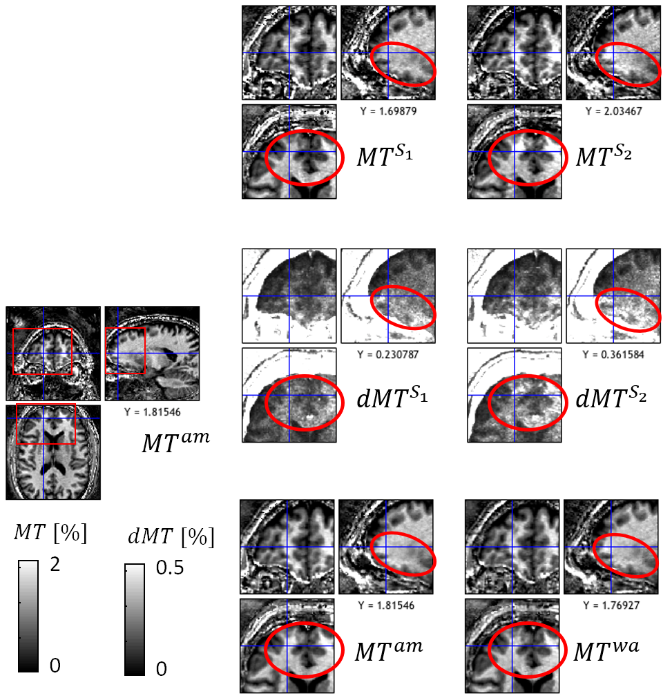
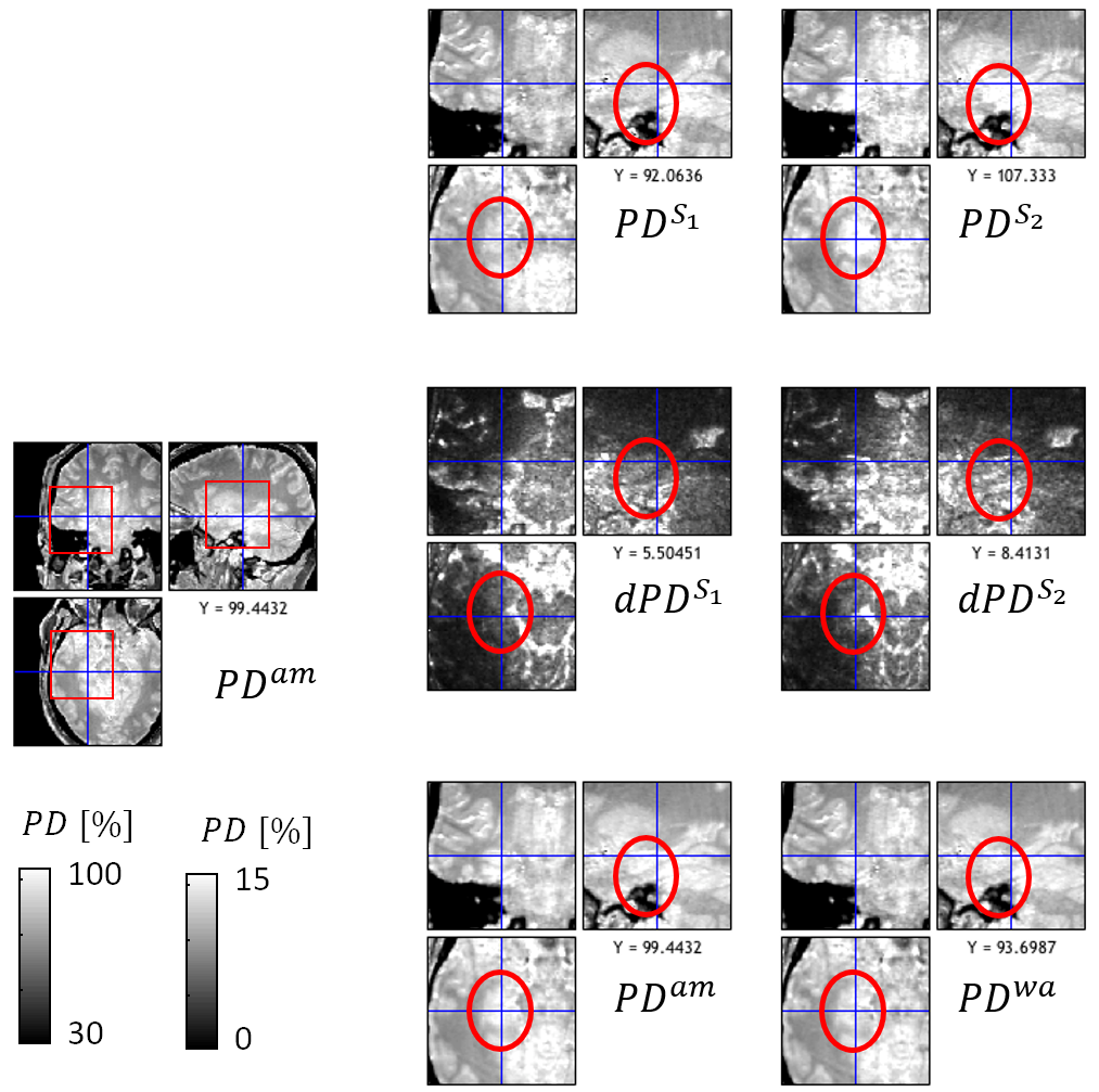
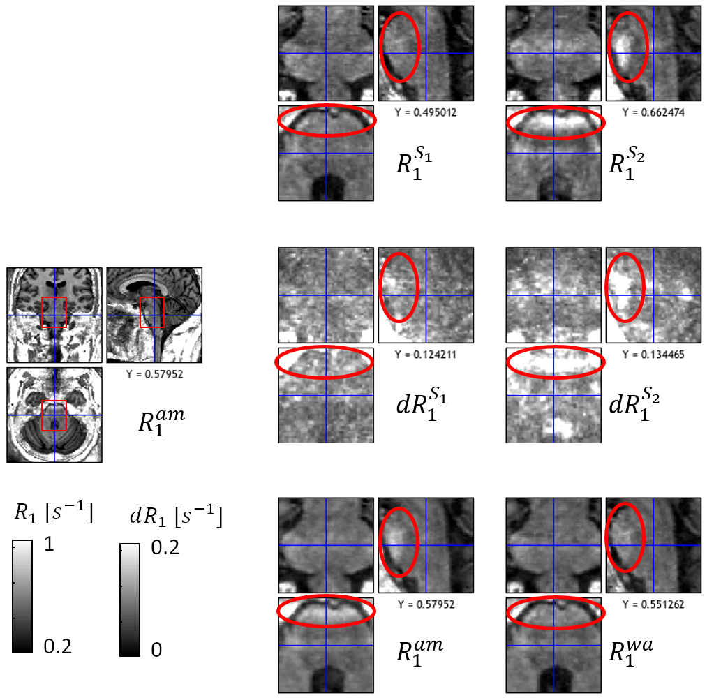
Step 3: The two runs (S₁,₂) of our measurement were combined using the arithmetic mean (superscript “am”) and a weighted average (superscript “wa”). For the example of R₁, the weighted-combination was defined as follows: $$(3) R_1 ^{wa} = \frac{R_1^{S1}f(ndR_1^{S1})+R_1^{S2}f(ndR_1^{S2})}{f(ndR_1^{S1})+f(ndR_1^{S2})} $$ where $$$ndR_1^{S1,2}=\frac{dR_1^{S1,2}}{dR_1^{S1}+dR_1^{S2}} $$$ and $$$f(x)=\frac{2}{exp((abs(x)-x_0)k_0)+1}$$$ being a Fermi function with two parameters ($$$x_0,k_0$$$), tuning the sensitivity of the weights with respect to the error in the data. Both parameters were heuristically optimized for one dataset that showed the worst motion artifacts.
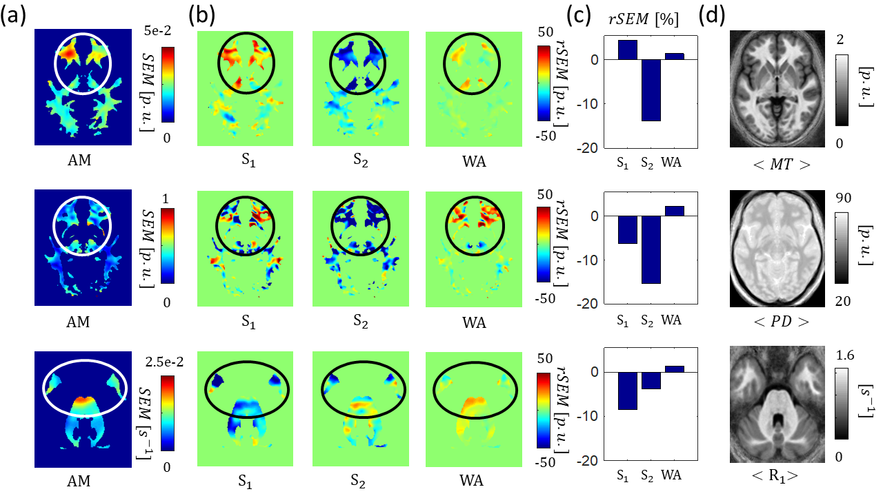
Group analyses: The hMRI toolbox⁷ was used to transform MPM maps into common space. Then, the variability across subjects was assessed by generating standard-error-of-the-mean (SEM) maps of each dataset (S₁, S₂, arithmetic mean, AM, and weighted average, WA) and MPM parameter (Fig.5a). The relative SEM with respect to the arithmetic mean ($$$rSEM=1-SEM_{inx}/SEM_{AM}$$$ with $$$inx=\{S_1,S_2,WM\}$$$) was calculated for all datasets. Since the bias introduced by subject motion and physiology increases the variability of the estimated parameters, positive rSEM values were interpreted as improved sensitivity for group differences.

Results

The proposed error maps (middle column, Fig.1) were more sensitive and specific to the artifacts in the different quantitative MPM maps (right column) than the regular model fit residuals from Eq. (1) (left column). Moreover, the error maps clearly differed between the different parameters (rows in Fig.1). We found for all three contrasts that the arithmetic mean of the proposed protocol showed less artifacts than each acquisition separately, both locally (Fig.2-4 and blue regions in Fig.5b with up to 50% improvement) and across the whole white matter (Fig.5c, up to 20%). In addition, the weighted average showed better performance than the arithmetic mean, both at a local (red regions in Fig.5b, up to 20%) and global level (Fig.5c, 1-3%).

Discussion and Conclusion

We introduced parameter specific error maps for the quantitative MPM maps (R₁, PD, MT) that are more specific and sensitive than previously introduced error maps (Eq. (1) and⁸). The error maps can be used to down-weigh erroneous regions. We found that their arithmetic average clearly improved the stability of the quantitative MPM maps, and that the proposed weighted-average further reduced variation. Future investigation will explore how the results generalize when larger cohorts are investigated and the suitability for patient groups.

Acknowledgements

This project was supported by LPEK_006_Kühn, by the ERA-NET NEURON (hMRI- ofSCI), the Bundesministerium für Bildung und Forschung (BMBF; 01EW1711A and B), and the Deutsche Forschungsgemeinschaft (grant MO 2397/4-1), and the Forschungszentrums Medizintechnik Hamburg (fmthh; grant 01fmthh2017).