1013
Data-driven Motion Detection for MR Fingerprinting1Siemens Healthcare GmbH, Erlangen, Germany, 2High Field MR Centre, Department of Biomedical Imaging and Image-guided Therapy, Medical University of Vienna, Vienna, Austria, 3Christian Doppler Laboratory for Clinical Molecular MR Imaging, MOLIMA, Vienna, Austria
Synopsis
In contrast to qualitative MRI, motion artifacts can be more subtle in quantitative MRI methods such as Magnetic Resonance Fingerprinting (MRF). Errors caused by motion are not easily detectable by visual inspection of resulting maps. Hence, there is clear need for supporting the reliability of results with regard to motion-induced errors. We present a method to detect if significant through-plane motion occurred during an MRF scan, without external motion tracking devices or acquiring additional data. The method is based on classifying the spatiotemporal residuals either by eye or a neural network. The performance was successfully evaluated in a patient study.
Purpose
Motion artifacts in MRI are usually accompanied by visible image artifacts. In quantitative MRI, results may be affected in a more subtle way: values in the parametric maps can be corrupted without obvious hints in the appearance of the maps1.Magnetic Resonance Fingerprinting (MRF)2 has a certain inherent robustness with regard to motion due to the applied pattern matching approach2. While MRF is indeed fairly insensitive to in-plane motion, several works suggest that 2D MRF is somewhat sensitive to strong through-plane motion3.4.
In this work, a method is presented to detect whether through-plane motion has occurred during a 2D slice-selective FISP-MRF5 experiment, purely based on analyzing the MRF signal course, i.e. without the need for external motion detection such as navigator scans or a camera.
Methods
We used a prototype implementation of FISP-MRF5 with a prescan-based6 B1+ correction and spiral sampling (undersampling factor 48, FoV 256 mm, resolution 1 mm, slice thickness 5mm) with a spiral angle increment of 82.5°7. 12 volunteers’ and 32 patients’ brains (suspicion of glioma) were scanned on 3T MRI scanners (MAGNETOM Prisma, MAGNETOM Prismafit and MAGNETOM Skyra, Siemens Healthcare, Erlangen, Germany).The motion detection method assumes that:
- the bulk movement of the head during the scan is rigid
- signal alterations due to motion have high frequency compared to the dictionary signals
- only signal alterations in solid matter are considered since e.g. fluid motion cannot be considered rigid
The residual maps from volunteer and patient scans were labelled manually as motion corrupted (type: nodding, tilting, or stretching; severity level 1,2, or 3) or not motion corrupted. An overall estimation of the motion impact that occurred in a slice can be calculated (non, low, medium, strong) from that.
In each of the 32 patients, at least 10 slices were scanned, once with FISP-MRF using 3000 TRs and twice with 1500 TRs. The difference of parameter values in ROIs in solid matter were calculated between the two 1500 TR acquisitions of the same slices and related to the detected motion. Across all patients and for each patient individually, the fraction of detected motion in the scanned slices was calculated.
Finally, a convolutional neural network was implemented to replace the manual classification of spatiotemporal residuals automatically. It was trained by using the manual classification of volunteer data and the data of 24 patients and tested on the data of the other 8 patients.
Results
Three distinct patterns can be observed when analyzing the spatial residuals. Deviations dominated by gradients in anterior-posterior direction are caused by a nodding-like motion. Tilting-like movements lead to similar gradients in left-right direction, and stretching causes an offset over the whole brain. These patterns occur with different strengths and are exemplarily depicted in Figure 2.Overall, no motion was detected in 77.0% of cases (i.e. slices), low motion in 8.8%, medium motion in 9.4%, and strong motion in 4.8% (Figure 3a)). This differs between unaffected scan sessions and strongly motion-corrupted ones (Figure 3b)).
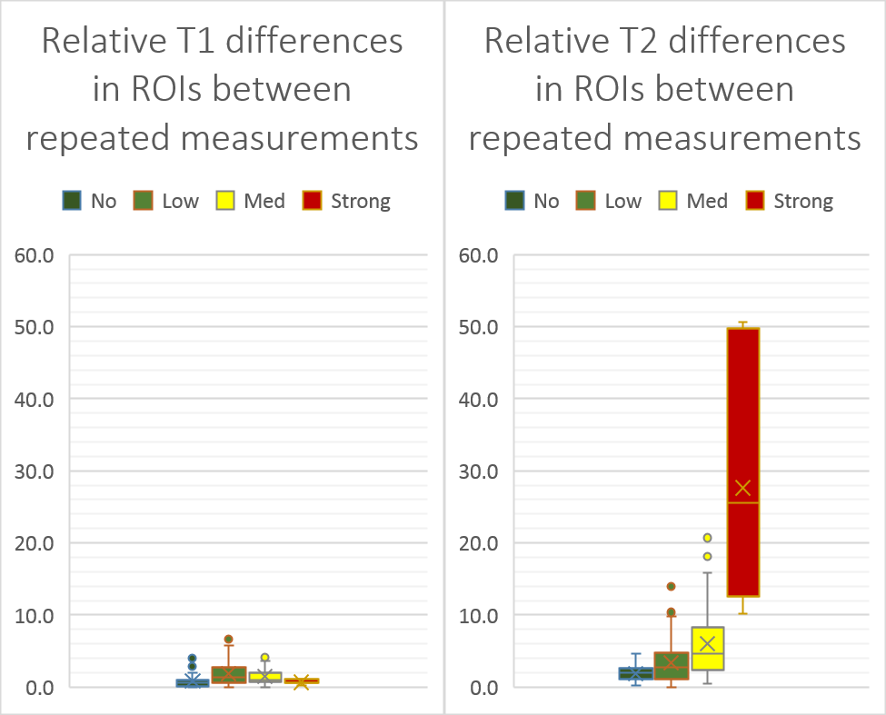
Relative T1 and T2 differences in solid-matter ROIs between repeated MRF scans using 1500 TR are depicted in Figure 4. The differences are grouped for cases with no motion in one repetition and in the other repetition also none, low, medium, or strong motion. The relative differences scale with the strength of the detected motion.
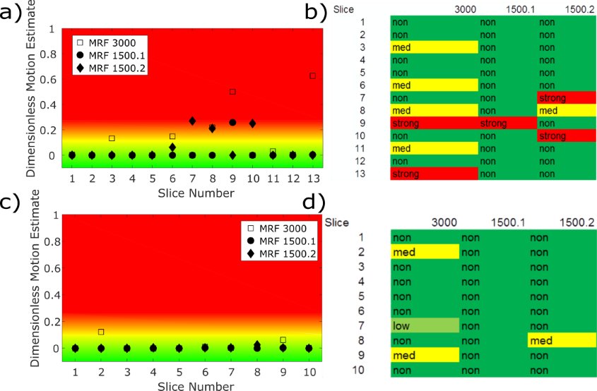
The neural net had an accuracy of 94.2% on single residual maps. The overall estimated motion per slice by the neural network and the corresponding manual assessment for two patients are presented in Figure 5.
Discussion & Conclusion
By analyzing spatiotemporal residuals, the impact of motion can be identified which is not reflected by similarity measures over the whole signal course such as the inner product. In consequence, this allows to highlight potential inaccuracies in the quantitative data. Our proposed approach is facilitated by the fact that brain motion can be considered as predominantly rigid.This novel method was successfully validated by comparing relative changes of T1 and T2 values to detected motions in repeated measurements. Results in a clinical study show that about 15% of the scanned data in patients were motion corrupted, while in some patients almost all data were corrupted and in some only a few slices.
Bulk motion artifacts can be superimposed by e.g. flow artifacts which makes simple fitting approaches unsuitable and requires to consider large brain area rather than single pixels. An approach to detect complex motion patterns is deep learning. The employed neural net had a high accuracy and was able to reproduce human estimations.
Future work is envisioned to provide more thorough validation by involving recorded motion data via e.g. an in-bore camera or artificially shifting and angulating the slice during the scan while the object/subject is kept still.
Acknowledgements
No acknowledgement found.References
1 Callaghan M. F. et al., An evaluation of prospective motion correction (PMC) for high resolution quantitative MRI, Front Neurosci. 2015
2 Ma D. et al, Magnetic resonance fingerprinting. Nature 2013;
3 Mehta G. et al, Image reconstruction algorithm for motion insensitive MR Fingerprinting (MRF): MORF, MRM 2018;
4 Yu Z. et al, Exploring the sensitivity of magnetic resonance fingerprinting to motion., MRI. 2018;
5 Jiang Y. et al, MR fingerprinting using fast imaging with steady state precession (FISP) with spiral readout. MRM 2015;
6 Chung S. et al, Rapid B1+ mapping using a preconditioning RF pulse with TurboFLASH readout, MRM 2010;
7 Körzdörfer G. et al, Effect of spiral undersampling patterns on FISP MRF parameter maps, MRI 2019
Figures
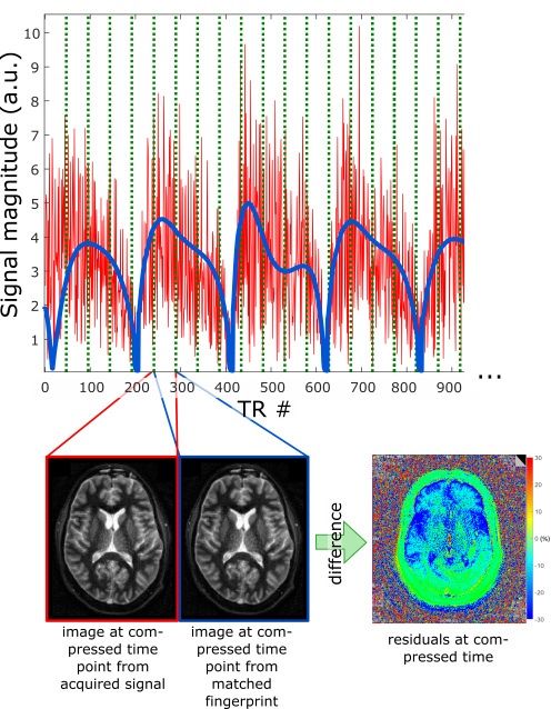
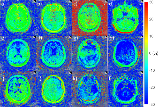
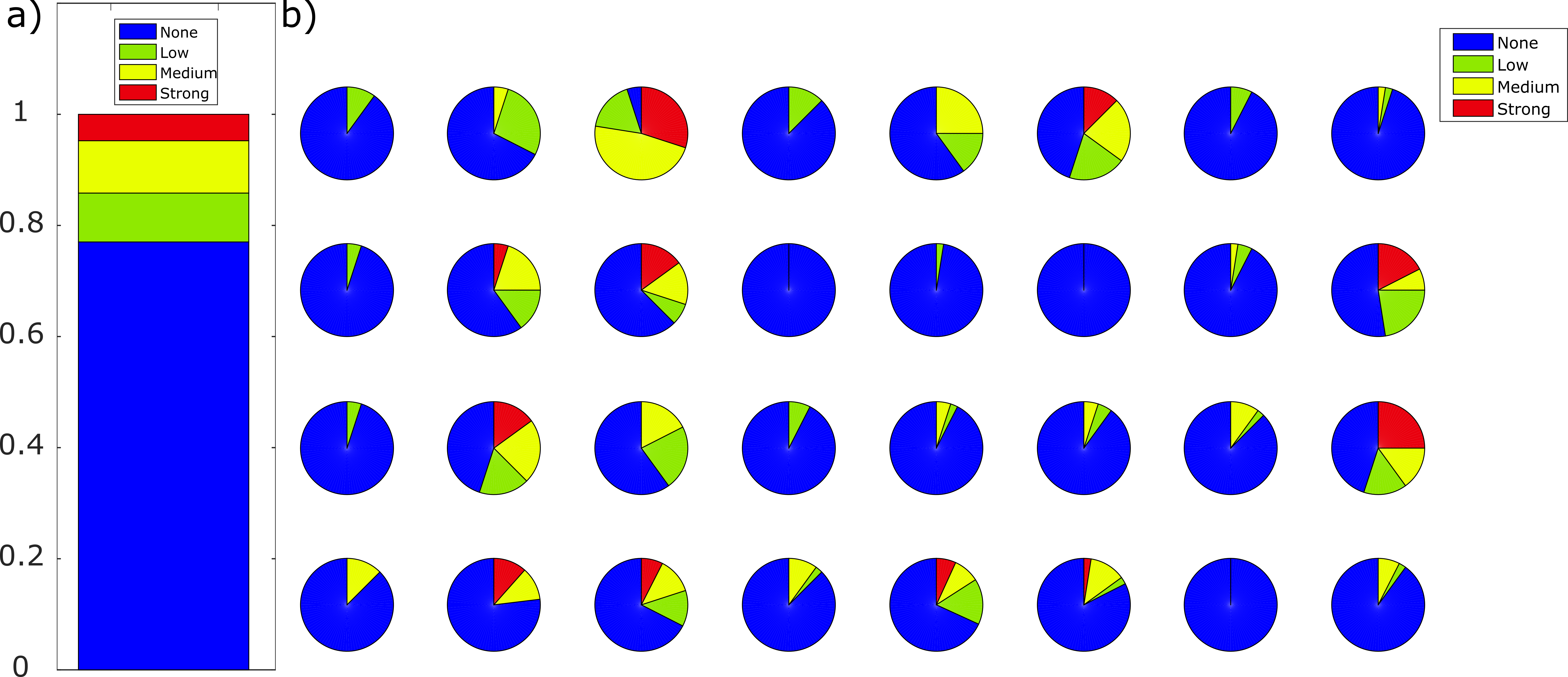
Figure 3: Fraction of detected overall motion levels per slice in all 32 patients is shown in a). In 77% of all measured slices no motion, in 8.8% low motion, in 9.4% medium motion, and in 4.8% strong motion was detected. In b) the fraction of overall motion per slice is depicted per patient.