1010
Myelin-sensitive Quantitative Maps: Two’s Company, Three’s a Crowd?
Matteo Mancini1,2,3, Eva Alonso-Ortiz2, Mara Cercignani1, Julien Cohen-Adad2, and Nikola Stikov2
1Department of Neuroscience, Brighton and Sussex Medical School, University of Sussex, Brighton, United Kingdom, 2NeuroPoly Lab, Polytechnique Montreal, Montreal, QC, Canada, 3CUBRIC, Cardiff University, Cardiff, United Kingdom
1Department of Neuroscience, Brighton and Sussex Medical School, University of Sussex, Brighton, United Kingdom, 2NeuroPoly Lab, Polytechnique Montreal, Montreal, QC, Canada, 3CUBRIC, Cardiff University, Cardiff, United Kingdom
Synopsis
Are myelin-sensitive maps interchangeable? We performed a scan-rescan study in 5 subjects using T1 mapping, magnetization transfer and myelin water fraction. We found overall that all metrics have high scan-rescan repeatability and that they are highly correlated with each other. However, isolating the main factor behind this shared variance is not straightforward because of the different interplays between the measures. In the end, what will matter is to what extent these relationships are preserved in the presence of pathology.
Introduction
One of the long-sought clinical applications of MRI is measuring myelin in vivo. Several modalities have been shown to be sensitive to it1. Common choices for myelin imaging include T2 relaxometry, magnetization transfer (MT) and T1 mapping. Are these techniques comparable in terms of scan-rescan reliability and more importantly do they provide equivalent measures? In this study we address this question focusing on four representative approaches: T1, estimated from the MP2RAGE2 sequence; MT saturation (MTsat), estimated using the multi-parameter mapping3 approach (MPM); MT ratio (MTR), also derived from MPM; and myelin water fraction (MWF), estimated using a 3D GRASE4 sequence.Methods
5 subjects (mean age(STD): 32.4(6.1), 3M/2F) were scanned twice on a Siemens Prisma 3T, using a tailored protocol that included: MPM3 based on stock (non-custom) sequences (three volumes: T1-weighted, PD-weighted, MT-weighted with 1.2 kHz off-resonance), MP2RAGE2, 3D GRASE4,5. The spatial resolution was 2 mm3 isotropic for all the sequences. Between the two acquisitions, each subject was taken out and put back in the scanner with repositioning.The MPM data was processed using SPM and the hMRI toolbox6 to reconstruct an MTsat map. From the hMRI-preprocessed MT-weighted and PD-weighted maps, the MTR was also computed. The MP2RAGE data was processed using publicly available code for T1 fitting developed by Marques and colleagues2. Finally, the GRASE data was processed using a dedicated pipeline provided by Lee and colleagues4 (version 1.4).The maps from the rescan sessions were rigidly registered to the respective ones from the first session using FSL FLIRT7 (version 6). The second inversion time volume from MP2RAGE was skull-stripped with FSL BET8 and processed with FSL FAST9 in order to extract a white matter mask. Finally, the data were aligned with the JHU white matter atlas10 registering the MNI template to each subject using a non-linear transformation estimated with ANTs11 (version 3.0.0). We selected 23 white matter ROIs, covering the main white matter structures (briefly, the corpus callosum, the corona radiata, the thalamic radiation, the sagittal stratum, the cingulum, the superior longitudinal fasciculus, the superior fronto-occipital fasciculus, and the uncinate fasciculus). For each measure, we computed the scan-rescan correlation both voxel-wise within the WM mask and across ROIs.
The relationships between the different measures were explored using scatterplots and 2D histograms first voxel-wise within the white matter mask and then at the ROI level. The Pearson correlation coefficient was used to quantify both the scan-rescan performance and the presence of linear relationships between each pair of measures. To further characterize relationships with a non-linear trend we used the polynomial fitting tools from the sklearn package12 (version 0.21.3).
Results
Fig. 1 shows the four maps for a sample subject. All the measures showed scan-rescan correlation higher than 0.8 (fig. 2a and fig. 3, main diagonal), with T1 and MTsat showing values higher than 0.9. The scatterplots and the related 2D histograms (fig. 3, upper triangle and lower triangle) show a linear trend between MTsat and T1, while the relationships between the other measures seem to be non-linear. When focusing on the ROIs, the scan-rescan correlation increases for MWF while it decreases for MTR (fig. 2a and fig. 4). Besides confirming the linear trend between MTsat and T1 (fig. 5), the ROI-based comparisons also highlight some non-linear trends, especially between MWF and T1: a quadratic regression analysis showed R2 scores of 0.768 and 0.662 respectively for MWF-T1 and MWF-MTsat, which are higher when compared to the linear fit (R2 scores of 0.70 and 0.57).Discussion
Although preliminary, these results indicate that the analysed measures are stable. An intriguing perspective is given by the strong linear relationship observed between T1 and MTsat. It seems that the reason behind this correlation may lie in the small MT effects observed in the stock MPM protocol, as shown by the relatively flat MTR map (most MTR values are between 0.25 and 0.3). The small dynamic range in MTR is also responsible for the poor correlations between MTR and each of the individual measures (see Fig. 2b), including MTsat from which it is derived. This is the reason why we excluded MTR from the ROI analysis.Future experiments are necessary to shed more light on our observations. We hypothesize that the small dynamic range in MTR from the MPM protocol is responsible for the high correlation between MTsat and T1. Acquiring a different MTR protocol with a higher offset frequency may give different results.
An important take-home message regarding MWF: as seen in the voxel-wise comparisons, MWF seems to be different from MT- and T1-based measures. However, one should take into account that MWF is noisier as seen from the voxel level scan-rescan correlations. Averaging over ROIs removes some of that noise and shows high agreement with MTsat and T1.
Conclusions
So can we substitute one myelin measure with another? At least in healthy white matter, it appears that the metrics are interchangeable, as figure 5 shows. However, when we look at more than two myelin-sensitive measures, the story gets more complicated. In the end, what will matter is to what extent these relationships are preserved in the presence of pathology.Acknowledgements
MM was funded by the Wellcome Trust through a Sir Henry Wellcome Postdoctoral Fellowship.References
- C. Laule et al. (2007), “Magnetic resonance imaging of myelin”, Neurotherapeutics, 4(3):460-84.
- J.P. Marques et al. (2010), “MP2RAGE, a self bias-field corrected sequence for improved segmentation and T1-mapping at high field“, Neuroimage, 49(2):1271-81.T.
- Weiskopf et al. (2013), “Quantitative multi-parameter mapping of R1, PD*, MT, and R2* at 3T: a multi-center validation”, Front Neurosci, 7:95.
- Prasloski et al. (2012), “Rapid whole cerebrum myelin water imaging using a 3D GRASE sequence”, Neuroimage, 63(1):533-9.
- J.Y. Choi et al. (2019), “Evaluation of Normal-Appearing White Matter in Multiple Sclerosis Using Direct Visualization of Short Transverse Relaxation Time Component (ViSTa) Myelin Water Imaging and Gradient Echo and Spin Echo (GRASE) Myelin Water Imaging”, J Magn Reson Imaging, 49(4):1091-1098.
- K. Tabelow et al. (2019), “hMRI - A toolbox for quantitative MRI in neuroscience and clinical research.”, Neuroimage, 194:191-210.
- M. Jenkinson and S.M. Smith (2001), “A global optimisation method for robust affine registration of brain images”, Med Image Anal, 5(2):143-156.
- S.M. Smith (2002), “Fast robust automated brain extraction”, Human Brain Mapping, 17(3):143-155.
- Y. Zhang et al. (2001), “Segmentation of brain MR images through a hidden Markov random field model and the expectation-maximization algorithm”, IEEE Trans Med Imag, 20(1):45-57.
- Mori et al. (2005), “MRI Atlas of Human White Matter”, Elsevier, Amsterdam, The Netherlands.
- B.B. Avants et al. (2008), “Symmetric diffeomorphic image registration with cross-correlation: evaluating automated labeling of elderly and neurodegenerative brain.”, Med Image Anal, 12(1):26-41.
- F. Pedregosa et al. (2011), “Scikit-learn: Machine Learning in Python”, JMLR, 12:2825-2830.
- A. Hagiwara et al. (2018), “Myelin Measurement: Comparison Between Simultaneous Tissue Relaxometry, Magnetization Transfer Saturation Index, and T1w/T2w Ratio Methods”, Sci Rep, 8(1):10554.
- M.N. Uddin et al. (2019), “Comparisons between multi-component myelin water fraction, T1w/T2w ratio, and diffusion tensor imaging measures in healthy human brain structures”, Sci Rep, 9(1):2500.
- S.Lévy et al. (2018), “Test-retest reliability of myelin imaging in the human spinal cord: Measurement errors versus region- and aging-induced variations”, PLoS One, 13(1):e0189944.
- Drenthen et al. (2019), “Applicability and reproducibility of 2D multi-slice GRASE myelin water fraction with varying acquisition acceleration”, NeuroImage, 195:333-339.
Figures
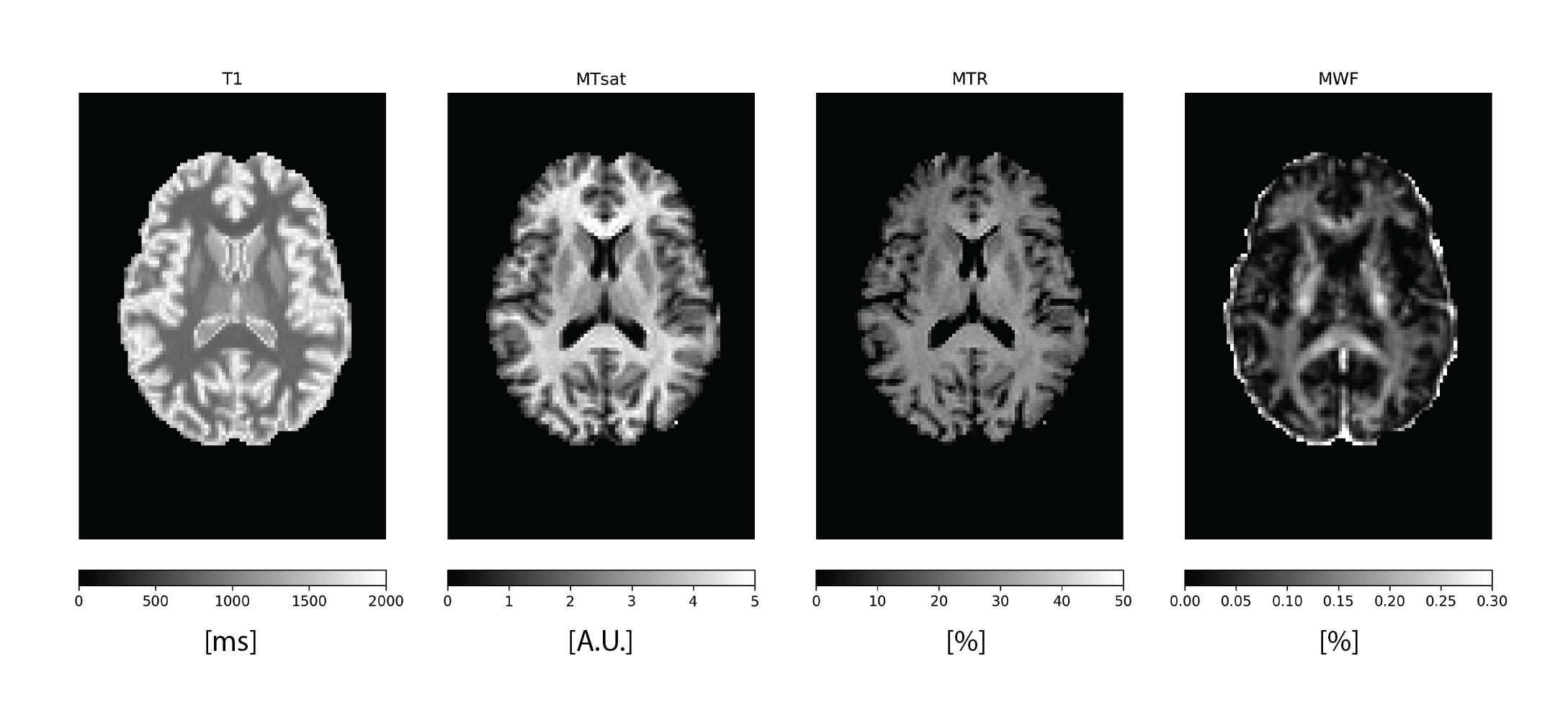
Figure 1. A selected axial slice of the four maps from one of the subjects.
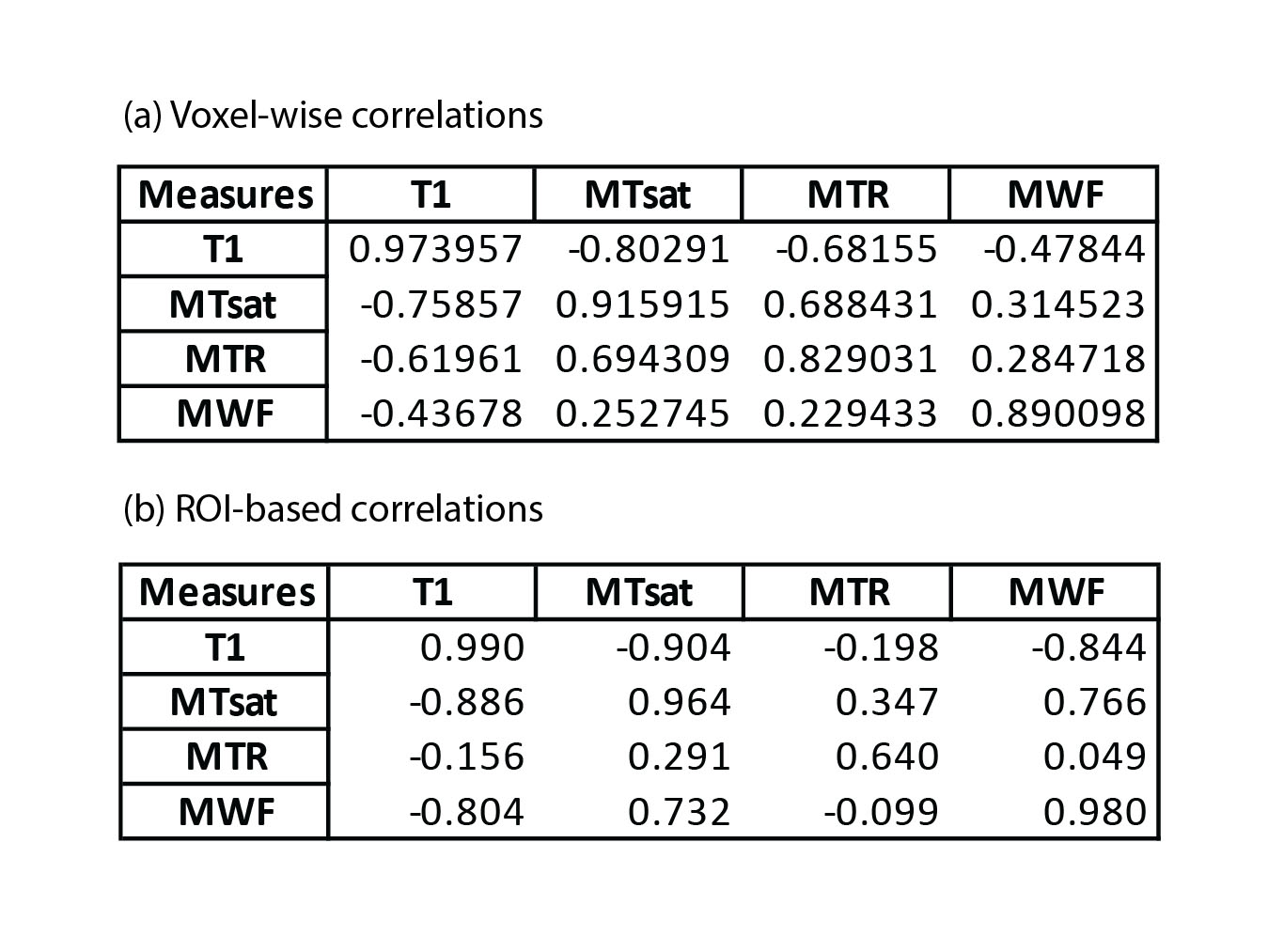
Figure 2. Scan-rescan and inter-modality Pearson correlation values for the voxel-wise analysis (a) and for the ROI-based one (b). The upper triangle of each table shows the correlations for the first session while the lower triangle shows the values for the rescan session. The diagonal shows the scan-rescan correlations.
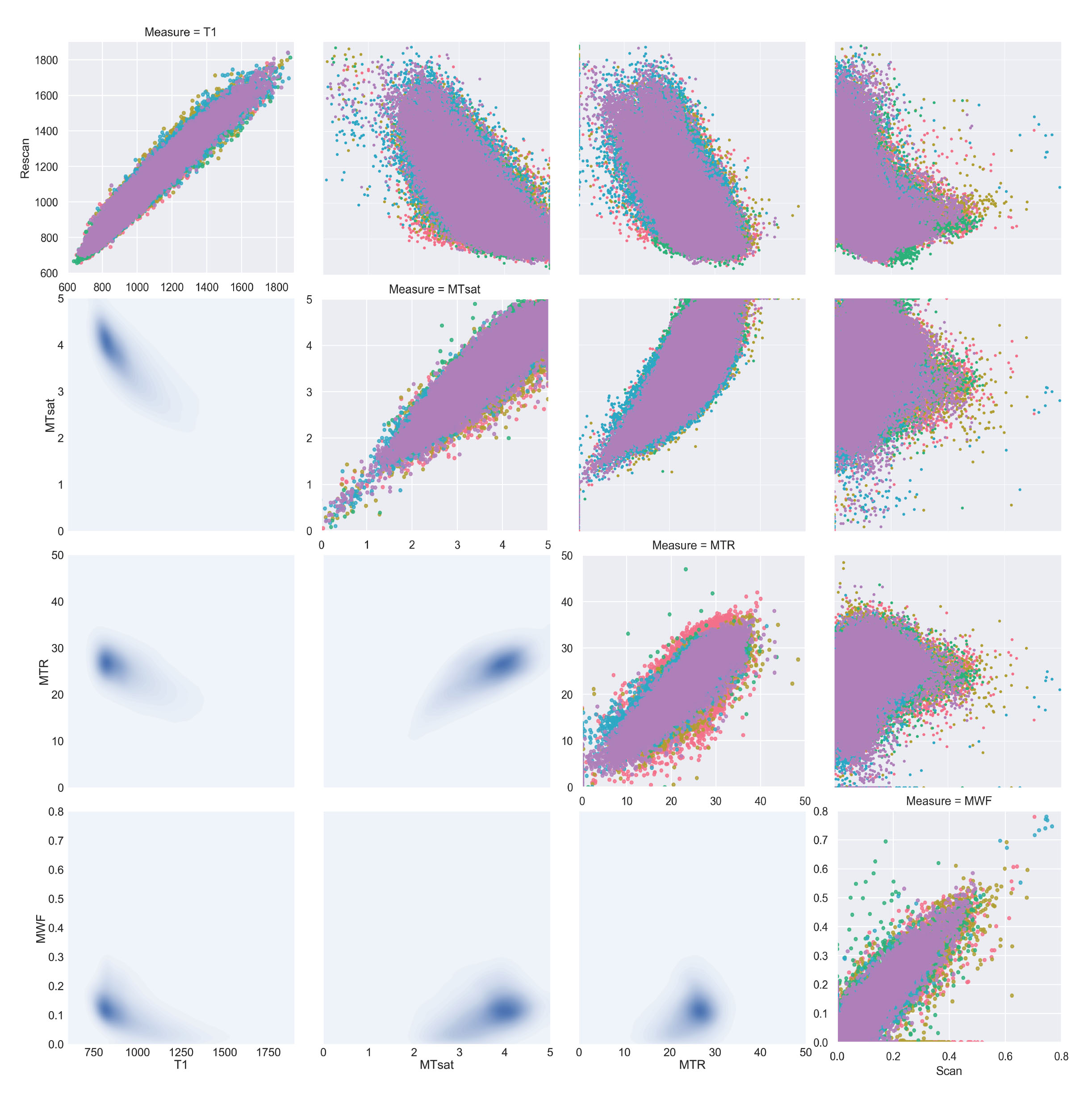
Figure 3. The voxel-wise scan-rescan for each metric is shown along the diagonal. The upper triangle shows voxel-wise scatter plots for each of the five subjects. In the lower triangle the data is pooled and displayed as a 2D histogram.
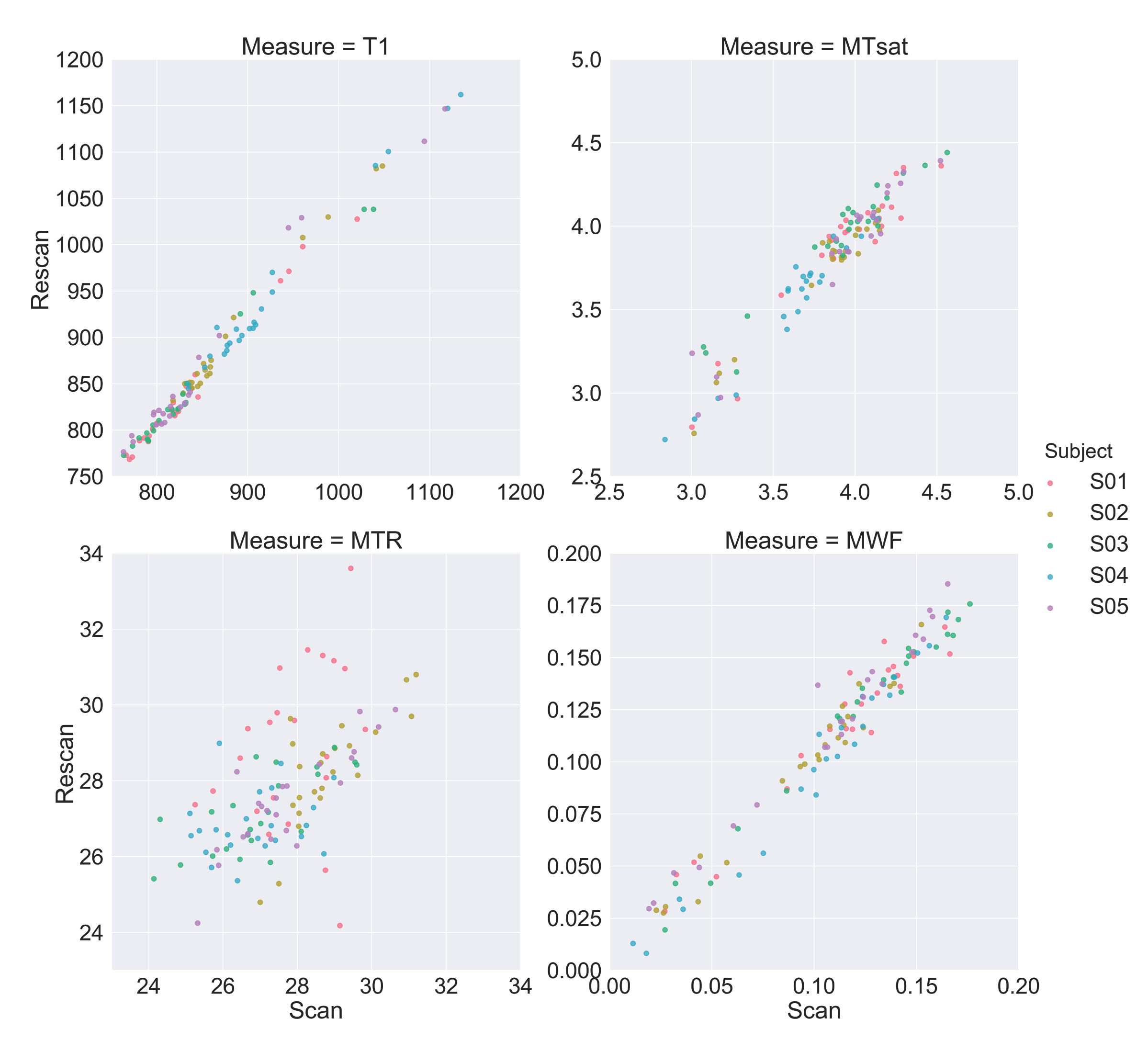
Figure 4. The ROI-based scan-rescan scatter plots for all the four measures.
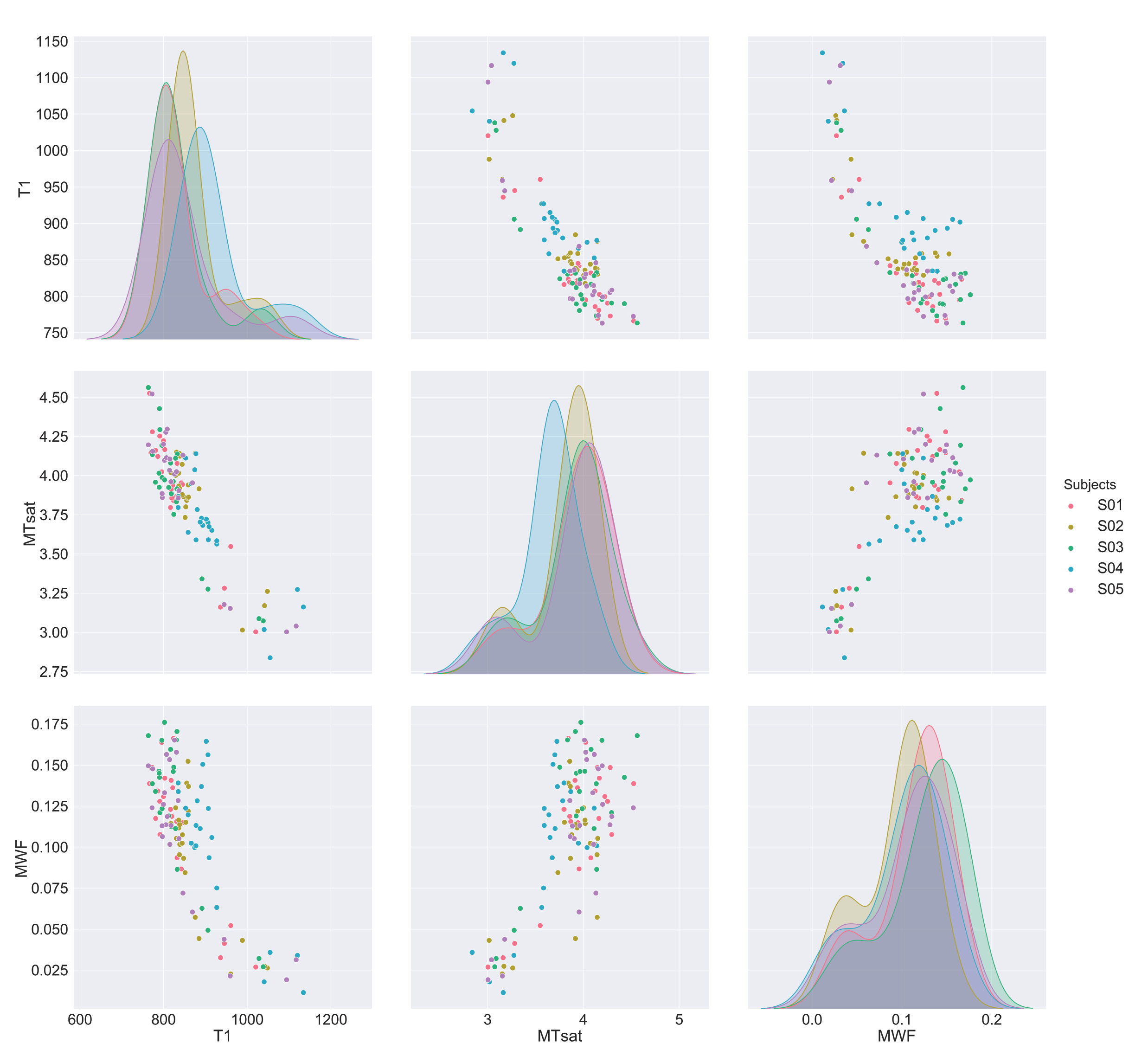
Figure 5. The off-diagonal scatter plots represent the relationships between each pair of measures, while the histograms on the diagonal show the distribution of each measure across the subjects.