0996
MRI Reconstruction Using Deep Bayesian Inference
Guanxiong Luo1 and Peng Cao1
1The University of Hong Kong, Hong Kong, China
1The University of Hong Kong, Hong Kong, China
Synopsis
A deep neural network provides a practical approach to extract features from existing image database. For MRI reconstruction, we presented a novel method to take advantage of such feature extraction by Bayesian inference. The innovation of this work includes 1) the definition of image prior based on an autoregressive network, and 2) the method uniquely permits the flexibility and generality and caters for changing various MRI acquisition settings, such as the number of radio-frequency coils, and matrix size or spatial resolution.
Introduction
In compressed sensing and parallel imaging MRI reconstruction, commonly used analytical $$$\ell_1$$$ and $$$\ell_2$$$ regularization can improve MR image quality1. Recently, deep learning reconstruction methods, such as cascade, deep residual, and generative deep neural networks have been used to optimize regularization or as alternatives to analytic regularization2–5. The density prior was used for reconstruction in Ref6. These methods have improved MR image reconstruction fidelity in some predetermined acquisition settings or pre-trained imaging tasks2–5. However, they are not robust for variable under-sampling schemes of MRI acquisition, such as the number of radio-frequency coils, and matrix size or spatial resolution. In this work, we apply Bayesian inference to the reconstruction problem, aiming to decouple the data-driven prior and the MRI acquisition settings.Methods
One of our motivations is to estimate a distribution over MR images that can be used to compute the likelihood of images and serve as a prior model for reconstruction. The generative network is commonly used to learn a parameterized model from images to approximate the real distribution7,8. We adopted PixelCNN++ as the prior model.With Bayes$$$'$$$ theorem, one could write the posterior as a product of likelihood and prior:$$f(\boldsymbol{x}|\boldsymbol{y}) = \frac{f(\boldsymbol{y}\mid\boldsymbol{x})g(\boldsymbol{x})}{f(\boldsymbol{y})} \propto f(\boldsymbol{y}\mid \boldsymbol{x} )\,g(\boldsymbol{x} )\label{eq:1},$$ where $$$f(\boldsymbol{y}\mid\boldsymbol{x})$$$ was probability of the measured k-space data $$$\boldsymbol{y}\in \mathbb{C}^M$$$ for a given image $$$\boldsymbol{x}\in \mathbb{C}^N$$$,where $$$N$$$ is the number of pixels and $$$M$$$ is the number of measured data points, and $$$g(\boldsymbol{x})$$$ was the prior model. The maximum a posterior estimation (MAP) could provide the reconstructed image $$$\hat{\boldsymbol{x}}$$$ , given by:$$\hat {\boldsymbol{x} }_{\mathrm {MAP} }(\boldsymbol{y})=\arg \max_{\boldsymbol{x}}f(\boldsymbol{x} \mid \boldsymbol{y})=\arg \max_{\boldsymbol{x}}f(\boldsymbol{y}\mid \boldsymbol{x} )\,g(\boldsymbol{x}). \tag{1}$$ The $$$n\times n$$$ image could be considered as an vectorized image $$$\mathit{\boldsymbol{x}} = (x^{(1)},...,x^{(n^2)})$$$, i.e., $$$x^{(1)}=x_{1,1}, x^{(2)}=x_{2,1},...,$$$ and $$$x^{(n^2)}=x_{n,n}$$$. The joint distribution of the image vector could be expressed as following :$$p(\boldsymbol{x};\boldsymbol{\pi,\mu,s, \alpha})=p(x^{(1)})\prod_{i=2}^{n^2} p(x^{(i)}\mid x^{(1)},..,x^{(i-1)}).$$$$$\boldsymbol{\pi,\mu,s,\alpha}$$$ were the parameters of mixture distribution for each pixel. Therefore, the network $$$\mathtt{NET}(\boldsymbol{x}, \Theta)$$$ shown in Figure 1(b), that predicts the distribution of all pixels of an image, was trained by$$\hat{\Theta} = {\underset {\Theta }{\operatorname {arg\,max}\ }}{ p(\boldsymbol{x}; \mathtt{NET}(\boldsymbol{x}, \Theta))},$$ where $$$\Theta$$$ was the trainable hyperparameters. When trained, the prior model $$$g(\boldsymbol{x})$$$ as $$g(\boldsymbol{x}) = p(\boldsymbol{x}; \mathtt{NET}(\boldsymbol{x}, \hat{\Theta})).\tag{2}$$ The measured k-space data $$$\boldsymbol{y}$$$ was given by$$\boldsymbol{y} = \mathbf{A} \boldsymbol{x} \ + \ \boldsymbol{\varepsilon},$$where $$$\mathbf{A}$$$ was the encoding matrix and $$$\boldsymbol{\varepsilon}$$$ was the noise. Substituting Eq. (2) into the log-likelihood for Eq. (1) yielded$$\hat{\boldsymbol{x}}_\mathrm{MAP}(\boldsymbol{y}) =\underset {\boldsymbol{x}}{\operatorname {arg\,max} }\,\log{f(\boldsymbol{y}\mid \boldsymbol{x} )} + \log{p(\boldsymbol{x}\mid \mathtt{NET}(\boldsymbol{x}, \hat{\Theta}))}. \tag{3}$$ The log-likelihood term $$${\log{f(\boldsymbol{y}\mid \boldsymbol{x} )}}$$$ had less uncertainties and was close to a constant with uncertainties from noise that was irrelevant and additive to $$$\boldsymbol{x}$$$. Hence, Eq. (3) can be rewritten as $${\hat {\boldsymbol{x} }}_{\mathrm {MAP} }(\boldsymbol{y}) = {\underset {\boldsymbol{x}}{\operatorname {arg\,max} }} \, \log{p(\boldsymbol{x}\mid \mathtt{NET}(\boldsymbol{x}, \hat{\Theta}))} \qquad \mathrm{s.t.} \quad \boldsymbol{y} = \mathbf{A} \boldsymbol{x} \ + \ \boldsymbol{\varepsilon}.$$ Then, the projected gradient method was used to solve above maximization, whose iterative steps were illustrated in Figure 1(c). The gradient was calculated by backpropagation.
For knee MRI, we used NYU FAST MRI reconstruction databases9. For brain MRI, we used a 3 T human MRI scanner (Achieva TX, Philips Healthcare) with an 8-channel brain coil for data collection. Fifteen healthy volunteers were scan by standard-of-care brain MRI protocols. (also put the scan parameters here if you have space)
Results
Our previous study used this method in different MRI acquisition scenarios, including parallel imaging, compressed sensing, and non-Cartesian reconstructions.Figure 2 shows the quantitative comparisons among the proposed method, GRAPPA, and compressed sensing10. The k-space used in comparisons were retrospectively under-sampled from the fully-acquired test data. Figure 3 shows the reconstruction results from prospectively accelerated data acquisition. Figure 4 shows the prior applied to spiral imaging. Figure 5 shows convergence curves reflected stabilities of iterative steps: 1) maximizing the posterior 2) k-space fidelity enforcement.
The same deep learning model has also been tested for various contrasts from other Cartesian k-space reconstruction experiments, thus there is no need to re-train the deep learning model for further studies.
Discussion
Our Bayesian method is a generic and interpretable deep learning-based reconstruction framework. It employs a generative network as the MRI prior model. The framework is capable of exploiting MRI data from the prior model, for any given MRI acquisition settings. The separation of the image prior and the encoding matrix embedded in the network made the proposed method more flexible and generalizable compared with conventional deep learning approaches.The proposed method can reliably and consistently recover the nearly aliased-free images with relatively high acceleration factors. The reconstruction from a maximum of posterior showed the successful reconstruction of the detailed anatomical structures, such as vessels, cartilage, and membranes in-between muscle bundles.
In this work, the results demonstrated the successful reconstruction of high-resolution image (256 x 256 matrix) with low-resolution prior (trained with 128 x128 matrix), confirming the feasibility of reconstructing images of different sizes without the need for retraining the prior model.
Conclusion
We presented the application of Bayesian inference in MR imaging reconstruction with the deep learning-based prior. The result demonstrated that the deep prior is effective for image reconstruction with flexibility in changing the MRI acquisition settings, such as the number of radio-frequency coils, and matrix size or spatial resolution.Acknowledgements
No acknowledgement found.References
- Lustig, Michael, David Donoho, and John M Pauly. “Sparse MRI: The application of compressed sensing for rapid MR imaging.” Magnetic Resonance in Medicine: An Official Journal of the International Society for Magnetic Resonance in Medicine 58.6(2007): 1182–1195.
- Aggarwal, Hemant K, Merry P Mani, and Mathews Jacob. “Modl: Model-based deep learning architecture for inverse problems.” IEEE transactions on medical imaging38.2 (2018): 394–405.
- Mardani, Morteza, et al. “Deep generative adversarial neural networks for compressive sensing MRI.” IEEE transactions on medical imaging 38.1 (2018): 167–179.
- Schlemper, Jo, et al. “A deep cascade of convolutional neural networks for dynamic MR image reconstruction.” IEEE transactions on Medical Imaging 37.2 (2017): 491–503.
- Sun, Jian, Huibin Li, Zongben Xu, et al. “Deep ADMM-Net for compressive sensing MRI.” Advances in neural information processing systems. 2016. 10–18.
- Tezcan, Kerem C., et al. "MR image reconstruction using deep density priors." IEEE transactions on medical imaging (2018).
- Gregor, Karol, et al. “Deep autoregressive networks.” arXiv preprint arXiv:1310.8499(2013). Print.
- Salimans, Tim, et al. “Pixelcnn++: Improving the pixelcnn with discretized logistic mixture likelihood and other modifications.” arXiv preprint arXiv:1701.05517 (2017).
- Zbontar, Jure, et al. “fastMRI: An Open Dataset and Benchmarks for Accelerated MRI.” CoRR abs/1811.08839 (2018). arXiv: 1811.08839. Web.
- Uecker, Martin, et al. “ESPIRiT an eigenvalue approach to autocalibrating parallel MRI: where SENSE meets GRAPPA.” Magnetic resonance in medicine 71.3 (2014): 990–1001.
Figures
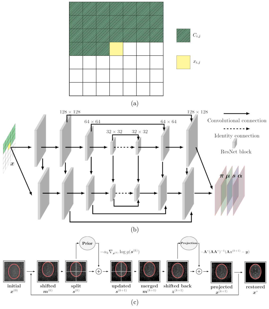
Figure 1. (a) The illustration of the conditional relationship. (b) Diagram shows the PixelCNN++ network in Ref8 which was the prior $$$g(\boldsymbol{x})$$$ used in this work. Each ResNet block consisted of 3 Resnet components. The input of network was $$$\boldsymbol{x}$$$, outputs were parameters of mixture distribution $$$(\boldsymbol{\pi, \mu, s, \alpha})$$$. (c) The prior $$$g(\boldsymbol{x})$$$ was trained with 128$$$\times$$$128 images. To address this mismatch, one 256$$$\times$$$256 image was split into four 128$$$\times$$$128 patches when applying the prior.
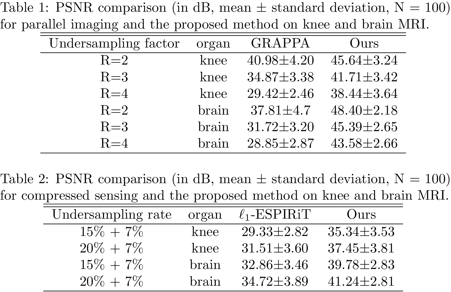
Figure 2. The quantitative comparisons. For both the knee imaging and brain imaging, 100 images (N=100) were used to test the performance of the proposed method via PSNR, which shows the proposed method provides huge improvements.
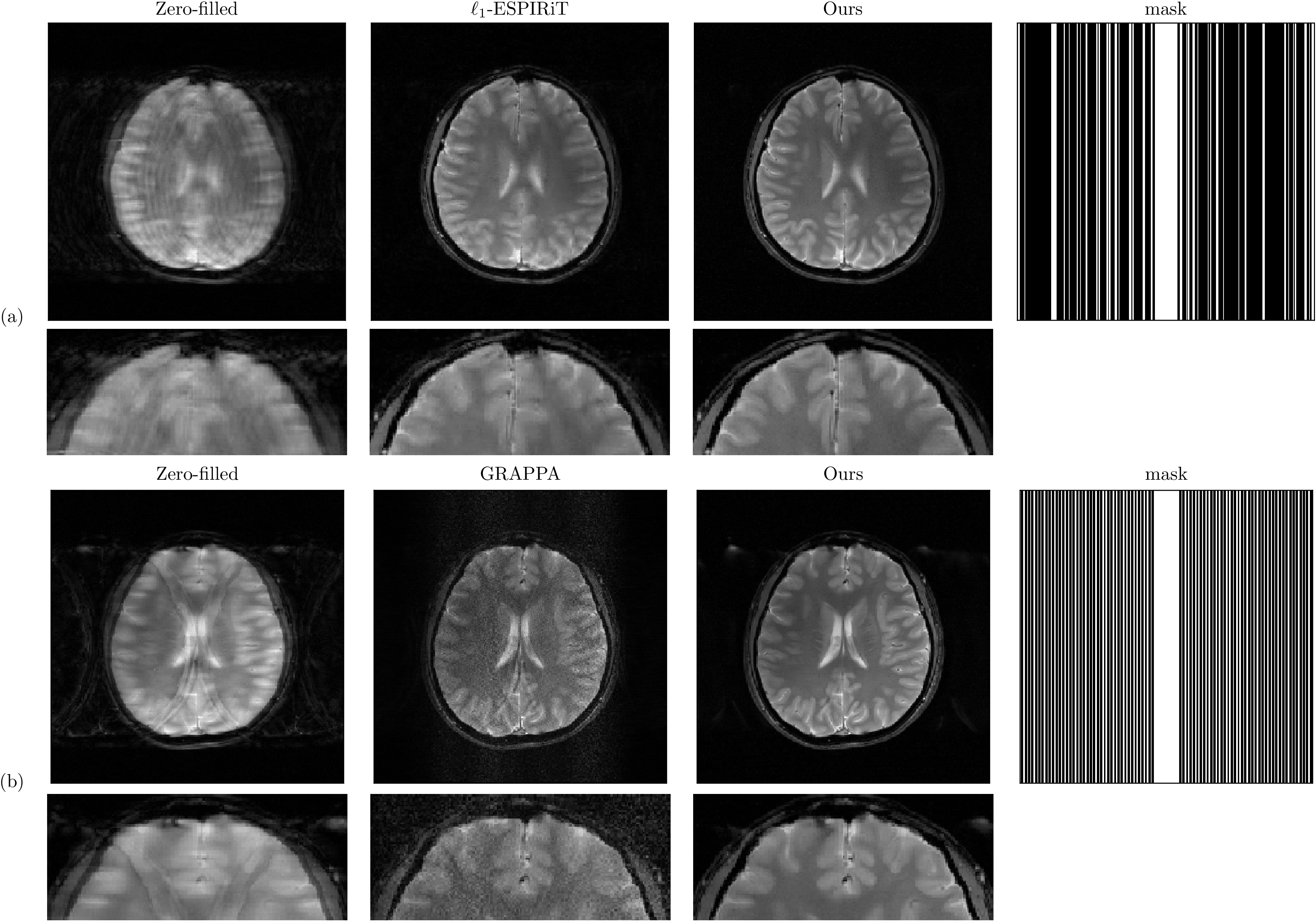
Figure 3. (a) Comparisons between compressed sensing and the proposed methods, using 22% k-space and 256$$$\times$$$256 matrix size, which shows the proposed method substantially reduced the aliasing artifact and preserved image details in compressed sensing reconstruction. (b) Comparisons between GRAPPA and the proposed methods under 3-fold acceleration. The proposed method effectively eliminated the noise amplification in GRAPPA reconstruction.
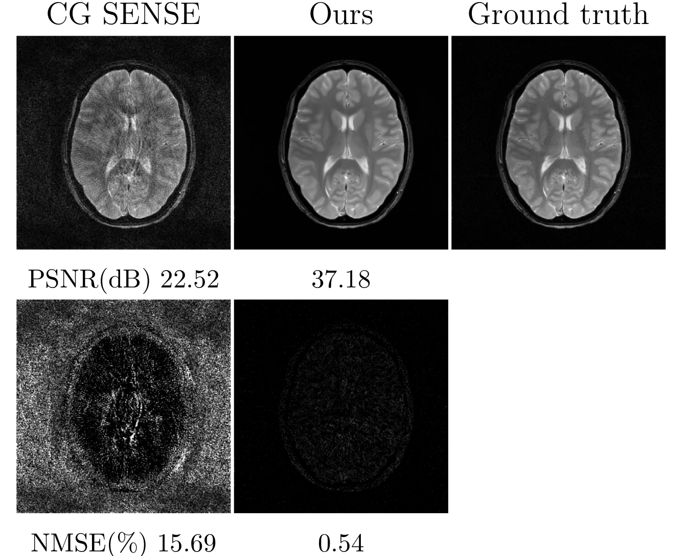
Figure 4. Comparison of the CG SENSE and proposed reconstruction for simulated spiral k-space with 4-fold acceleration (i.e., 6 out of 24 spiral interleaves), acquired T2$$$^∗$$$weighted gradient echo sequence. The intensity of error maps was five times magnified. The proposed method substantially reduced the aliasing artifact in spiral reconstruction. Noted that the same deep learning model used in the previous Cartesian k-space reconstruction was applied to spiral reconstruction, without the need of re-training the deep learning model.
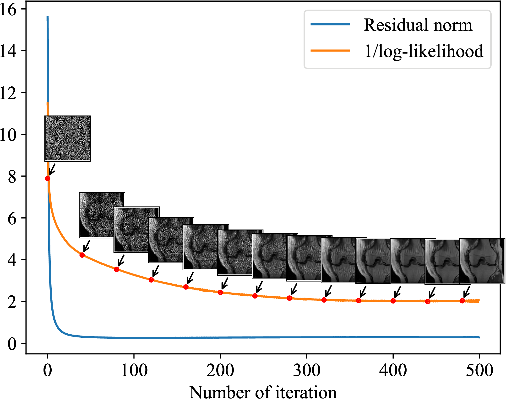
Figure 5. The 22% sampling rate and 1D undersampling scheme were used in this simulation. The residual norm was written as $$$\|\boldsymbol{y}-\mathbf{A}\boldsymbol{x}\|_2^2$$$, and the reciprocal of log-likelihood for MRI prior model was given in Eq. (2). The decay of residual norm stopped earlier than that of the log-likelihood. This evidence indicated that using the residual norm as the $$$\ell_2$$$ fidelity alone was sub-optimal, and the deep learning-based statistical regularization can lead to a better reconstruction result compared with the $$$\ell_2$$$ fidelity.