0995
A spatially adaptive cross-modality based three-dimensional reconstruction network for susceptibility imaging1Xiamen University, Xiamen, China
Synopsis
In this work, we propose a spatially adaptive cross-modality based three-dimensional reconstruction network to determine the susceptibility distribution from the magnetic field measurement. To compensate the information lost in previous encoder layers, a set of spatially adaptive modules in different resolutions are embedded into multiscale decoders, which extract features from magnitude images and field maps adaptively. Thus, the magnitude regularization is incorporated into the network architecture while the training stability is improved. It is potential to solve inverse problems of three-dimensional data, especially for cross-modality related reconstructions.
Introduction
Due to the singularity at the magic angle in the dipole convolution kernel, reconstruction of the magnetic susceptibility distribution from local phase is an ill-conditioned inverse problem. In image reconstruction tasks, network design should be wary of normalization, because that may result in loss of image contrast and intensity information. However, when training deep networks without any normalization, certain problems are prone to occur, such as gradient vanishing, gradient explosion, overfitting. In this work, we design a spatially adaptive module (SAM) and embed it to decoder layers, aiming to provide supplementary information for normalized feature maps. In particular, magnitude images and field maps are input to SAM in separate channel and subsequently their features are learned and combined adaptively. Hence, the network can eliminate the risk of information loss in encoder layers, meanwhile enable to apply batch normalization (BN)1 for the training stability.Methods
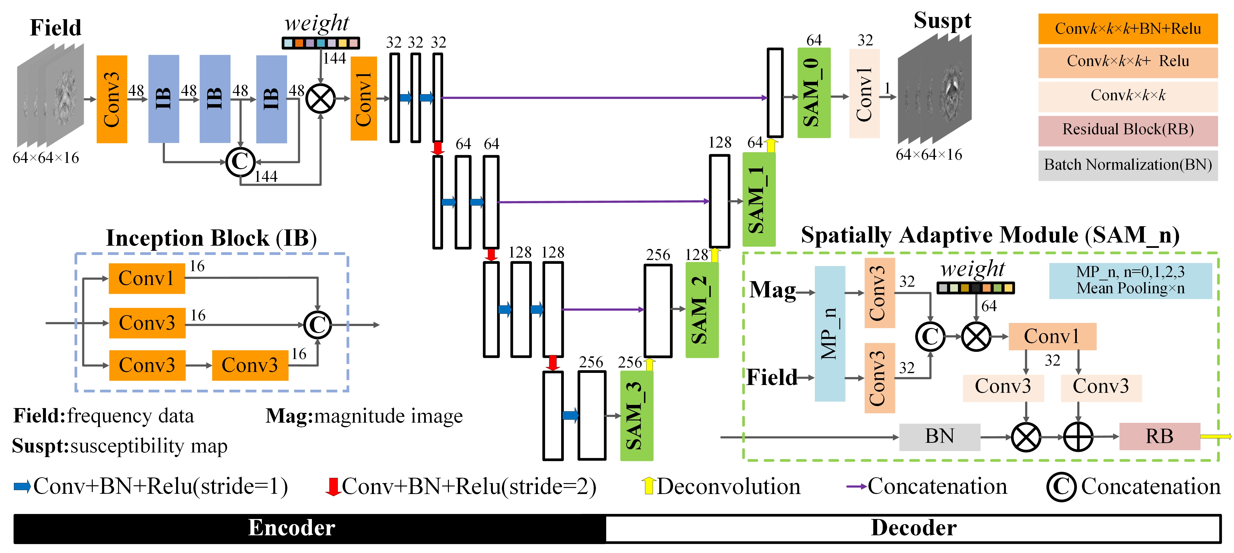
The proposed network is a multiscale framework containing subnets of encoder and decoder and all convolution kernels are in 3D dimension as illustrated in Fig. 1. Considering the computation limit, magnitude and field data is cropped into patches of size 64×64×16.In the encoder part, three inception blocks (IB)2 are employed and their learned multilevel features are concatenated and fused by a trainable weighting vector3. In detail, each IB block will perform convolution of three different sizes and the next block will determine how the obtained feature maps are used. Compared to a fixed value in common U-net4, this structure has a dynamic receptive field in the range of 3 to15. These feature maps are input to the subsequent encoder layers for further coding so that the network can extract more multiscale and multilevel features.
In the decoder section, SAM, composed of spatially adaptive normalization5 and residual block6, is introduced to the last layer before each deconvolution step. Unlike other BN methods, SAM is a conditional normalization, where weighting parameters are defined as spatial tensors instead of a vector, which is capable to extract features from magnitude and field data adaptively. The residual block is explored to reinforce fine structures by stretching texture residuals.
Experiment
Our training data contains 20 scans from nine healthy subjects acquired at a 7T MRI. Each subject was scanned in four directions with 9-16 echoes, TR/TE1/DTE=45/2/2ms, FOV=220×220×110, matrix size=224×224×110, taking COSMOS results as label data. The loss function used to train the network is defined according to mean absolute error and gradient loss terms7. The network was trained with 30 epochs over 10 hour on the Tensorflow deep learning framework using ADAM optimizer. The computing system is equipped with 32×Intel Xeon E5-2620 CPU, one 12 GB GTX 1080Ti GPU, and 128 GB RAM.We evaluated the network performance on susceptibility reconstructions using healthy adult brain, hemorrhage patient and numerical simulation data with calcification, to assess the overfitting problem in generalization. All network parameters are trained using the in vivo healthy data and have no additional fine-tuning or transfer learning in other data applications. Our network was compared to methods of simple TKD, optimization-based SFCR8 and conventional U-net, where the threshold in TKD is 0.2 and parameters in SFCR are set to be λ1=50, λ2=1, γ1=2000, γ2=20.
Results
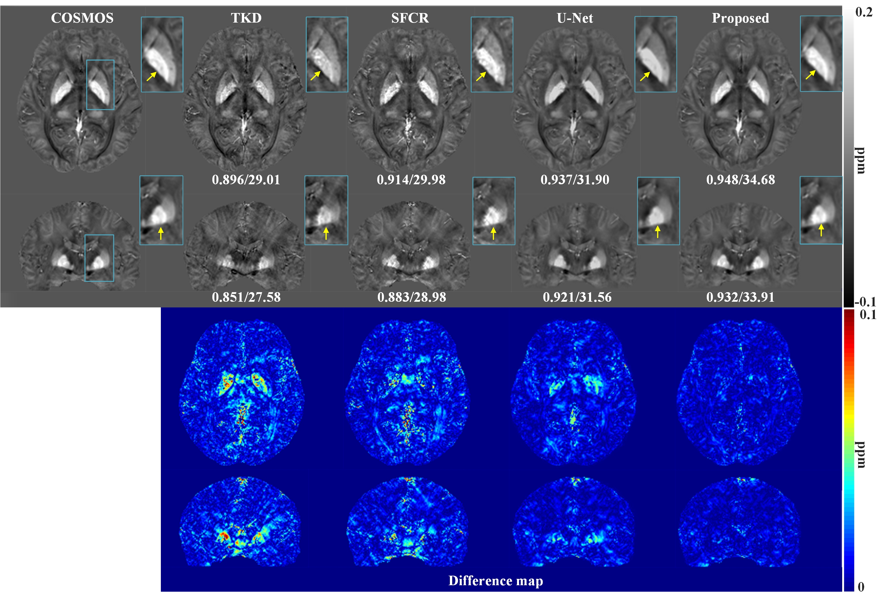
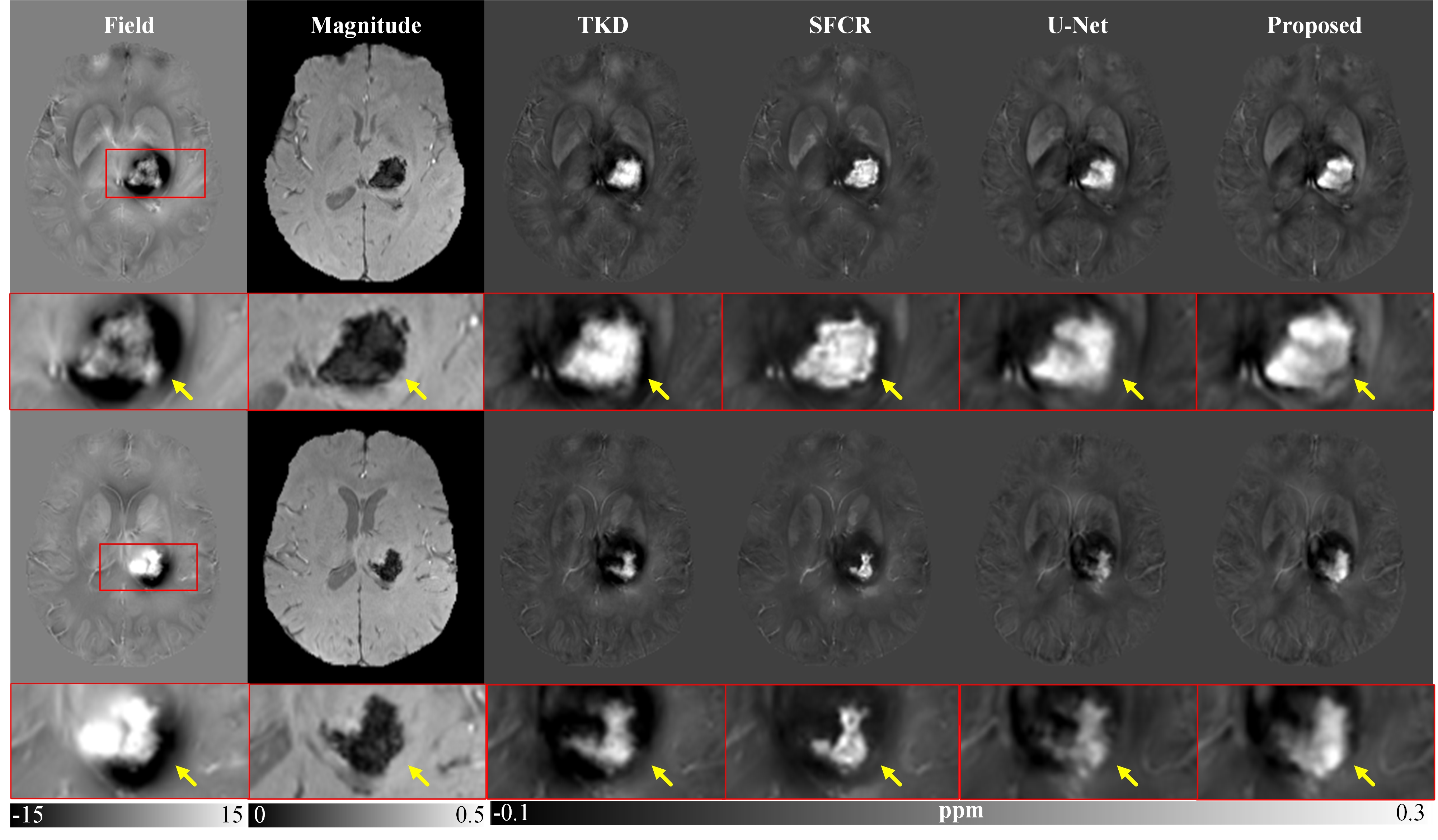
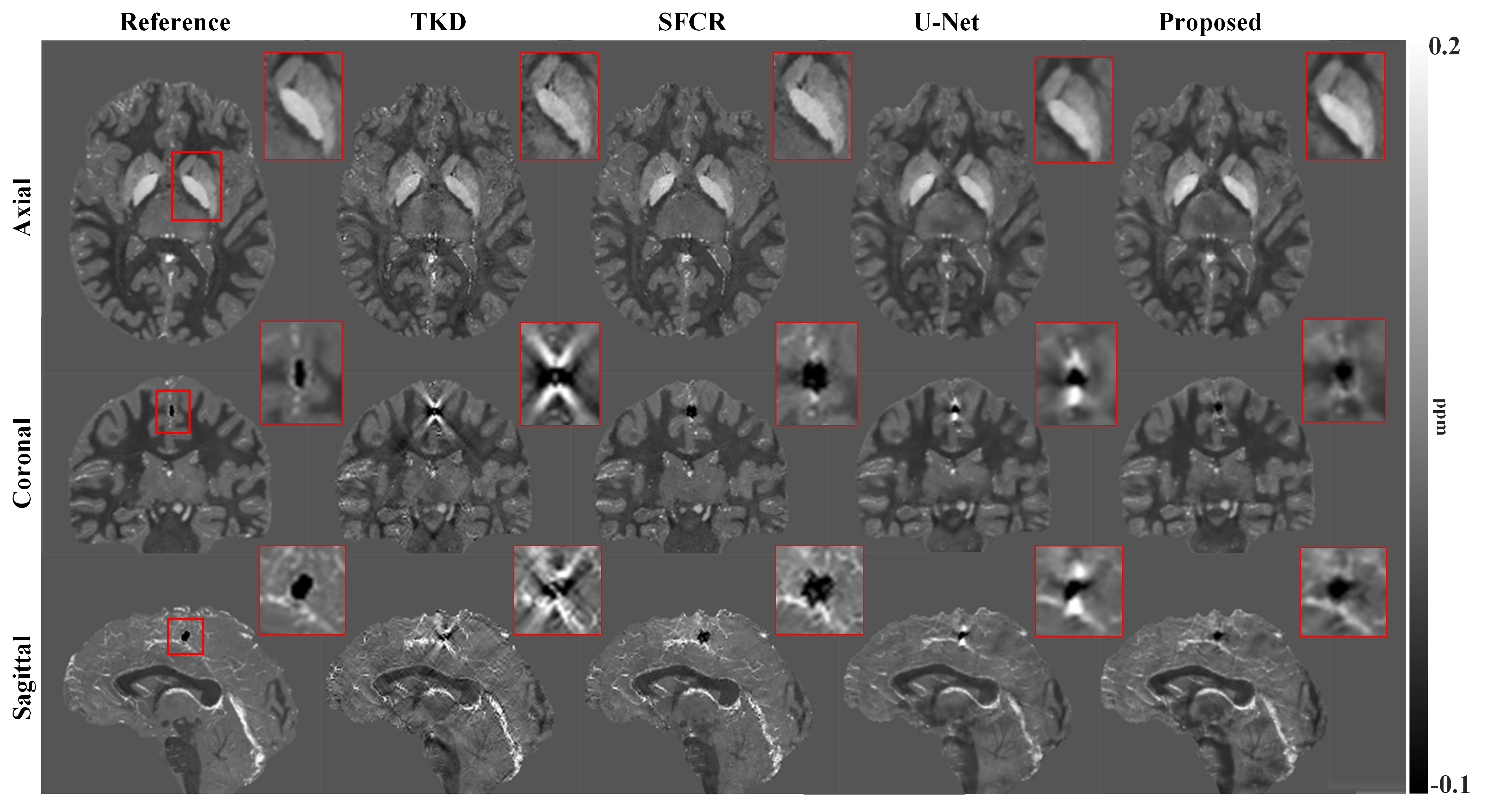
Figure 2 shows susceptibility maps reconstructed using different methods. The result of our method can recover the finest details and the sharpest contrast, e.g. boundaries between gray matter, white matter and cerebrospinal fluid, cerebral gyri and blood vessels, with the least artifact and the highest PSNR/MSSIM scores. Besides, there are smallest errors in corresponding difference maps. Figure 3 presents clinical application in brain hemorrhage data. Compared to the magnitude image, in the field map we can see serious susceptibility artifacts around the hematoma area. Suffering from these artifacts, the susceptibility maps generated from other methods cannot clearly recover the ROI boundary. However, our results incorporate the cross-modality pathological information and achieve a more reliable susceptibility map. Figure 4 illustrates the results on 2019 QSM reconstruction challenge data. We can see that our network can successfully recover the calcification region, but other methods fails to suppress the significant streaking artifacts caused by large susceptibility variations. Moreover, different levels of susceptibility contrast between tissues are exactly reconstructed and most close to the ground truth.Discussion
Due to the singularity at the magic angle in the dipole kernel, reconstruction of the susceptibility distribution from local phase is an ill-conditioned inverse problem, a priori magnitude based regularization is always used to facilitate the susceptibility estimation. The deep learning needs to learn a nonlinear mapping between the field shift and susceptibility distribution. Unlike to the undersampled MRI reconstruction, here the network convolution kernels should be three dimensional and the network input, i.e. field data, could not be normalized. In addition, the magnitude constraint is required to be implemented in a functional module. Therefore, we proposed a spatially adaptive cross-modality based three-dimensional network and then validate it on susceptibility imaging. Experimental results have demonstrated that the magnitude regularization is effectively incorporated into the network architecture while the training stability is improved. It is potential to solve inverse problems of three-dimensional data, especially for cross-modality related reconstructions.Acknowledgements
This work was supported in part by NNSF of China under Grant 81301277, Natural Science Foundation of Fujian Province of China 2019J01047.References
1. S. Ioffe, C. Szegedy, Batch Normalization: Accelerating deep network training by reducing internal covariate shift, arXiv:1502.03167 (2015) https://arxiv.org/abs/1502.03167.
2. Szegedy C, Vanhoucke V, Ioffe S, Rethinking the inception architecture for computer vision, Proc. IEEE CVPR (2016) 2818-2826.
3. Hu J, Shen L, Sun G, Squeeze-and-excitation networks, Proc. IEEE CVPR (2018) 7132-7141.
4. Ronneberger O, Fischer P, Brox T, U-Net: Convolutional networks for biomedical image segmentation, Proc. MICCA I (2015) 234-241.
5. Park T, Liu M Y, Wang T C, Semantic image synthesis with spatially-adaptive normalization, Proc. IEEE CVPR (2019) 2337-2346.
6. He K, Zhang X, Ren S, Sun J, Deep residual learning for image recognition, Proc. IEEE CVPR (2016) 770–778
7. Nie D, Trullo R, Lian J, Medical image synthesis with deep convolutional adversarial networks, IEEE Trans. Biomed Eng. 65 (2018) 2720-2730.
8. Bao L, Li X, Cai C, Quantitative Susceptibility Mapping using Structural Feature based Collaborative Reconstruction (SFCR) in the Human Brain, IEEE Trans Med. Imaging 35 (2016) 2040-2050.
Figures