Introduction

Undersampling is often necessary to reduce MRI scan time and cope with motion, but it leads to an ill-posed inverse problem. Reconstructing the true image requires perceptual criteria that capture an expert radiologist’s perception of acceptable images. Such criteria are complex to model. Learning from training data has been commonly adopted to define perceptual metrics. However, it often requires supervised training with a large and specific set of label images, consisting of fully-sampled high-quality images. Collecting such label images is expensive or impossible for scenarios such as dynamic imaging. On the other hand, 2D scans for static body parts are often fully-sampled with high enough quality to serve as labels. To cope with a small label set or leverage a large but different label set, semi-supervised (i.e. unpaired) training is the method of choice. To develop unpaired training schemes with minimal supervision, we leverage Wasserstein Generative Adversarial Networks (WGANs)¹. WGANs improve the training stability of GANs² and avoid the mode collapse issues associated with standard GANs². We present experiments and comparisons across various objectives for paired and unpaired training of neural networks (NNs) for MRI reconstruction.

Methods

Diagrams illustrating the training flow for both paired and unpaired cases are shown in Fig. 1. We use an unrolled network as our generator (G), the network performing the reconstruction, shown in Fig. 2. The unrolled network can be envisioned as a state-space model which at the $$$k$$$-th iteration takes an image estimate $$$x_k$$$, moves it towards the affine subspace of data consistent images, then applies a proximal operator (i.e. a neural network in our case), to obtain $$$x_{k+1}$$$. The state-space model can expressed as $$v_{k+1}=g(x_k),\ x_{k+1} = NN(v_{k+1}),$$ where $$$g$$$ is data consistency (DC) with a learnable step size $$$\mu$$$:$$g(x)=x+\mu\ \Big[\sum_{i=1}^c\mathcal{F}^{-1}\big\{\Omega\odot\mathcal{F}\{x\odot s_i\}\big\}\odot s_i^H-x_{\rm zf}\Big],$$where $$$x_{\rm zf}$$$ is the naive reconstruction of the k-space masked by $$$\Omega$$$ and $$$s_i$$$ are the coil sensitivities.

The discriminator network (D) is a plain convolutional NN (see Fig.1). It assigns a score to each of its input, which is as low as possible on generated data, and as high as possible on real data. Two channels are used to represent real and imaginary parts of the complex-valued images. The training objectives for the D and G are, respectively:

$$\min_{\Theta_D}\mathbb{E}\big[D(x;\Theta_D)\big]-\mathbb{E}\big[D({y};\Theta_D)\big]+\eta\mathbb{E}\big[(\| \nabla_{\hat{\hspace{0.7mm}x}}D(\hat{\hspace{0.7mm}x};\Theta_D)\|_2-1)^2\big],$$ $$\min_{\Theta_G}-(1-\lambda)\mathbb{E}\big[D(G({x_{\rm zf}};\Theta_G);\Theta_D)\big]+\lambda\mathbb{E}\big[\big\|{y}-G(x_{\rm zf};\Theta_G) \big\|_1\big],$$where $$$x$$$ is the G output, $$$y$$$ is the fully-sampled image, $$$\hat{\hspace{0.7mm}x}$$$ is drawn uniform randomly between $$$x$$$ and $$$y$$$, $$$\eta$$$ and $$$\lambda$$$ are hyper-parameters controlling the gradient penalty and $$$\ell_1$$$ loss weights, respectively.

In the unpaired case, $$$\lambda=0$$$, and D can take single-channel magnitude images: an option in addition to that in the paired case. We explore this relaxation so that datasets which only consist of magnitude images and no k-space data can also be used as labels. Without the $$$\ell_1$$$ term, the objectives for the unpaired case is the WGAN-GP³ loss, which minimizes the Wasserstein-1 distance between the real and generated image distribution. WGAN offers more stable training than other GANs because Wasserstein-1 distance is continuous everywhere while distances (e.g. JS divergence or, $$$\chi^2$$$ divergence) minimized by other GANs^2,4 becomes infinity when the distributions are disjoint. Image distributions are in high-dimensional spaces and often disjoint.

Experiments

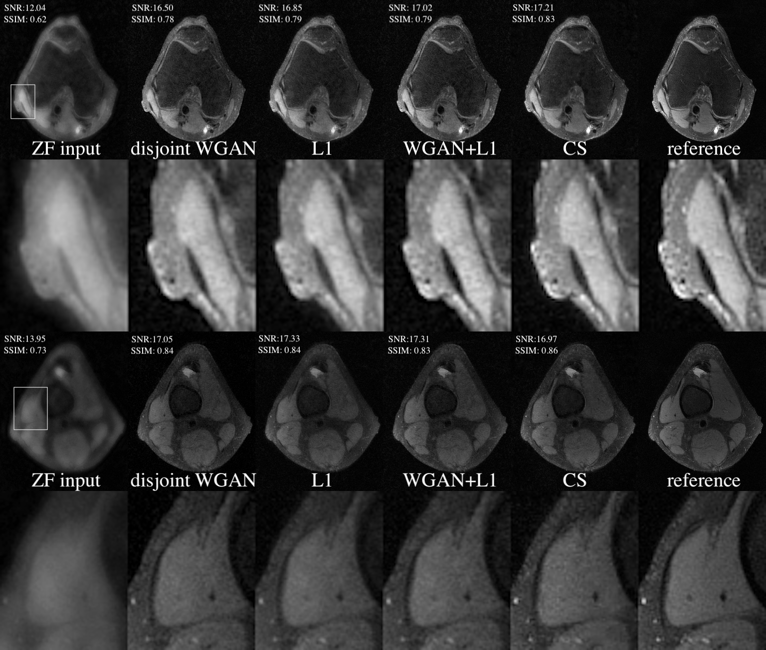
Unpaired training. Besides using partial labels, we explore a more relaxed version of unpaired training, disjoint, where there is no overlap between the input and label sets. Undersampled k-space data from 7 subjects are used as inputs, and fully-sampled magnitude images from other 6 subjects are used as labels. This setting is useful when we want to train a model for a dataset with any label using high-quality labels from some other datasets.

Paired training. We consider a supervised scenario with input and label pairs from 6 subjects. The network is trained with WGAN+$$$\ell_1$$$ loss or only $$$\ell_1$$$ loss.

Compressed sensing with Wavelet regularization (CS-WV)⁵ reconstructed images are presented as a comparison. Its regularization parameter is manually tuned for best perceptual quality on a small evaluation set.

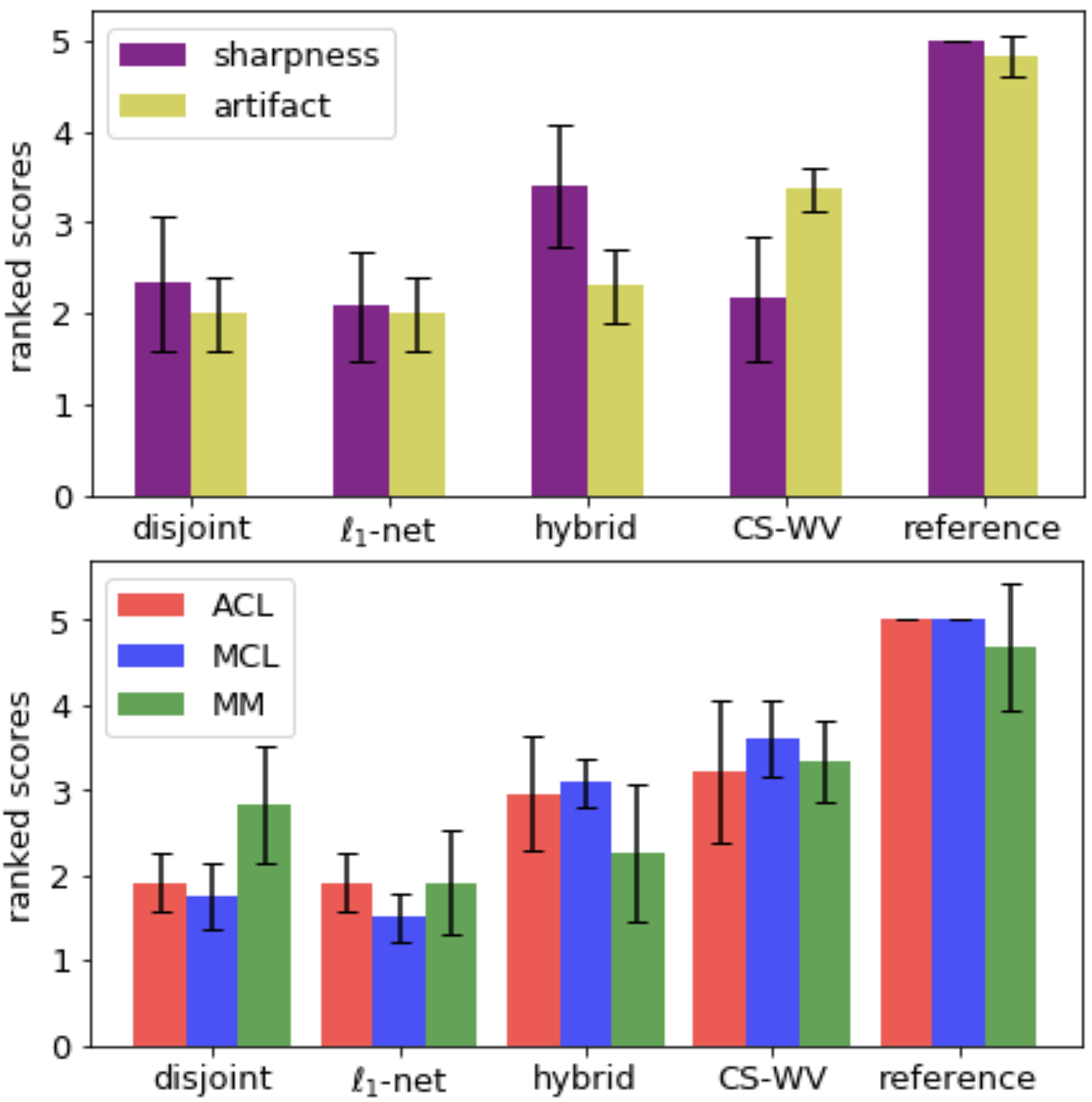
Two test slices from the above four methods are shown in Fig. 3, and the quantitative scores (averaged across six test volumes) are shown in Table 1. Two radiologists rated each reconstructed volume from five aspects and the scores are shown in Fig. 4. When paired training is possible, adding WGAN objective to the classic $$$\ell_1$$$-minimization leads to results that are visually sharper with higher SNR. Otherwise, one can use the proposed unpaired training which gives comparable results.

Reconstruction time. Our unrolled G takes 0.025 seconds (averaged across two test volumes) to reconstruct one 2D slice. A 30-iteration CS-WV reconstruction takes 0.4 seconds per slice.

Conclusion

We introduce an unpaired deep learning scheme for MRI reconstruction when high-quality training labels are scarce. Leveraging WGANs, a generator network maps linear image estimates to mimic the image label distribution. The proposed unpaired training alleviates the need for pairing among undersampled inputs and diagnostic quality labels. We also show that for paired learning scheme, additional WGAN objectives improves the reconstruction quality. The best of our NN models are 16x faster and arguably better than CS. Extensive experiments on MRI knee datasets corroborate the efficacy of WGANs with an unrolled generator in faithful reconstruction of MRIs.

Acknowledgements

Work in this paper was supported by the NIH R01EB009690 and NIHR01EB026136 award, and GE Precision Healthcare.