0985
Rapid Boundary Artifacts Correction for Simultaneous Multi-slab (SMSlab) Acquisition Using Convolutional Network1Center for Biomedical Imaging Research, Department of Biomedical Engineering, School of Medicine, Tsinghua University, Beijing, China
Synopsis
Simultaneous multi-slab (SMSlab) technique is a 3D acquisition method that can achieve optimal signal-to-noise ratio (SNR) efficiency for high-resolution diffusion-weighted imaging (DWI) or functional MRI (fMRI). However, boundary artifacts may restrain its application. Nonlinear inversion for slab profile encoding (NPEN) has been proposed for its correction, which needs long computation time. In this study, we propose to use a convolutional network for boundary artifacts correction. It can solve the problem in a short time and improve the signal-to-noise ratio (SNR), which is of great meaning for high-resolution whole-brain DWI and fMRI.
Introduction
Simultaneous multi-slab (SMSlab) acquisition1 is a combination of simultaneous multi-slice (SMS) and 3D multi-slab techniques. In SMSlab, multiple 3D slabs are excited simultaneously to achieve the optimal signal-to-noise ratio (SNR) efficiency. In this way, it enables the acquisition of 3D high-resolution diffusion weighted images or functional MR images2.However, a remaining challenge, boundary artifacts, restrain the application of this technique3-5. It mainly results from truncated RF pulses and introduces intra-slab intensity variation and inter-slab aliasing. Several methods were proposed to correct for boundary artifacts for multi-slab acquisition3,4,6,7. They can suppress the artifacts when the repetition time (TR) is long enough. Only nonlinear inversion for slab profile encoding (NPEN)3,8 can solve the problem at TR = 2000 ms, but its computation is time-consuming. It won’t be practical when a large number of brain volumes are acquired.
After being trained by a sufficient amount of high-quality data, a convolutional network (CNN) can solve a complex inverse problem in 1 second9. Therefore, in this work, we investigate the ability of CNN to correct for boundary artifacts for the SMSlab acquisition.
Methods
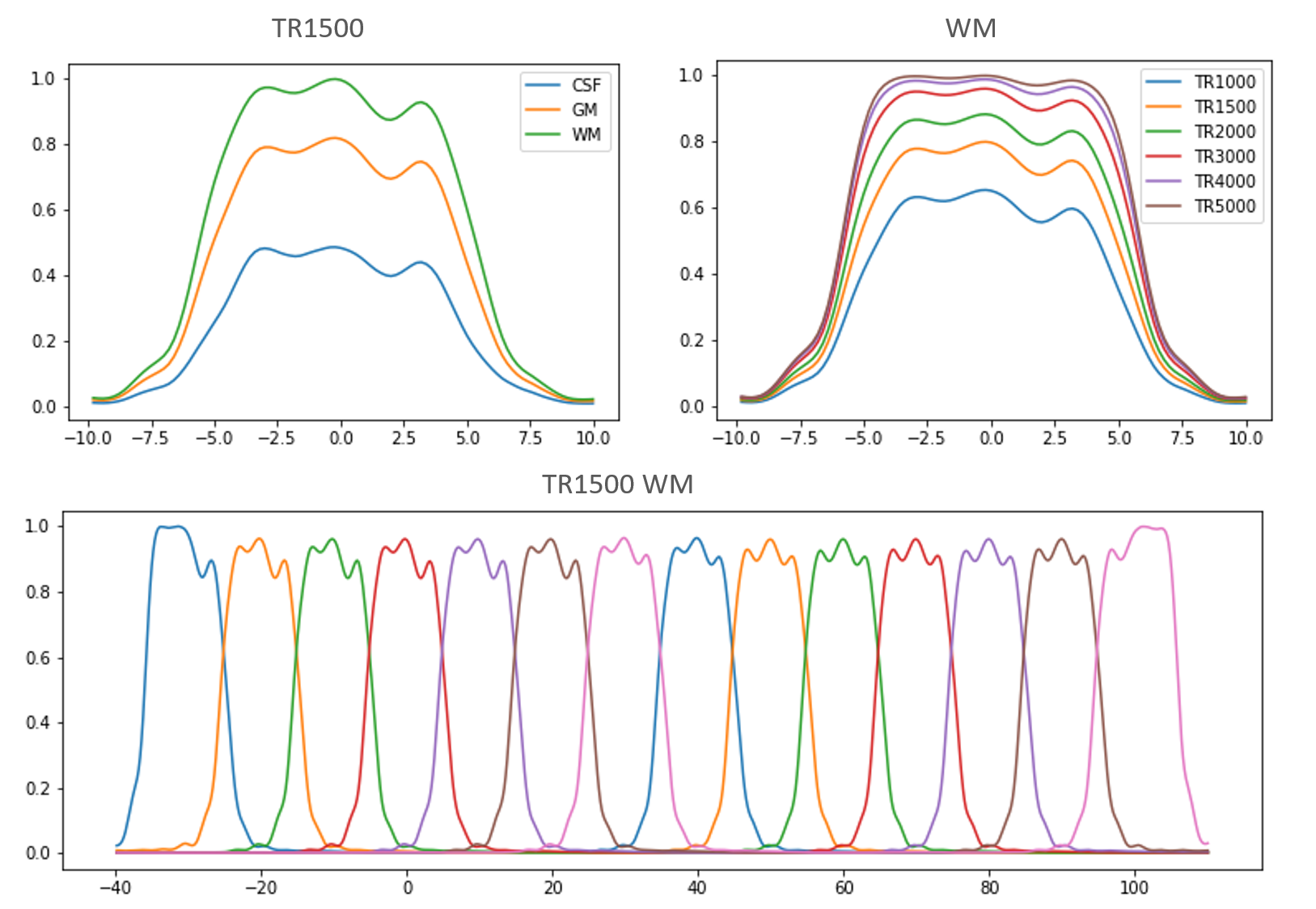
Bloch simulation was used to generate slab profiles of the SMSlab sequence1. 2 slabs were excited simultaneously (MB factor = 2). A 12-mm slab thickness was used. Each slab contained 12 slices, 2 of which were overlapped with the neighboring slabs. The slab thickness used in the refocusing pulse was 1.17 times as large as that of the excitation pulse. An interleaved slab ordering was used. The simulation was repeated with TR values ranging from 1000 ms to 5000 ms on gray matter (GM), white matter (WM), and cerebrospinal fluid (CSF) because they are different in T1.Ten subjects were taken from the Human Connectome Project (HCP) 10, which contains DWI data. Only 1 volume of non-DWIs (b = 0 s/mm2) and 1 direction of DWIs (b = 1000 s/mm2) of each subject were extracted for training. Images of 6, 3, and 1 subjects were used for training, validation, and test, respectively. Each volume contained 140 slices, which were divided into 7 x 2 (MB factor) = 14 slabs.
By multiplying the reference images with the simulated slab profiles at different TRs (TR = 1000, 1500, 2000, 3000, 4000, 5000 ms), and then creating inter-slab aliasing on the simultaneously excited slabs (Fig. 2b), images with different levels of boundary artifacts were created. For GM, WM, and CSF, corresponding slab profiles were used. The tissue segmentation was finished using FAST from the FMRIB software library (FSL)11. To imitate the SNR which decreases as the TR is shortened, Gaussian white noise was added to reach a maximum level of 10 dB at TR = 1000 ms.
The convolutional network used in this study was a modification of U-net12, a network widely used for image segmentation. Its depth was reduced to 3 and only 8 filters were used in the first layer of the network. The model was trained by Adam optimizer13 with the structural similarity index (SSIM) loss14.
The training set and validation set contained synthetic images at all TRs except for TR = 1000 ms, which served as the test data. The images with artifacts and the slab profiles were used as input, and reference images were used as output. For further evaluation of the results, fractional anisotropy (FA) maps were calculated using FDT from FSL11. The NPEN algorithm refined for the SMSlab acquisition1,8 was used for comparison in this study.
Results and Discussion
Fig. 1 shows the results of the Bloch simulation. As TR decreases, the magnitude decreases because of insufficient T1 recovery. Slab crosstalk leads to intensity reduction at the edges of slabs. The slab profiles vary for different kinds of tissue. The longitudinal magnetization of tissue with shorter T1 (WM) is recovered better.The synthetic artifacts are shown in Fig. 2a. Image contrast changes between different TRs. Intensity inhomogeneity at slab boundaries becomes more severe and SNR drops when TR is shortened. In DWIs, the SNR is lower, but the artifacts are less severe because the signal of CSF is suppressed. Fig. 2b shows the aliasing pattern of the SMSlab acquisition.
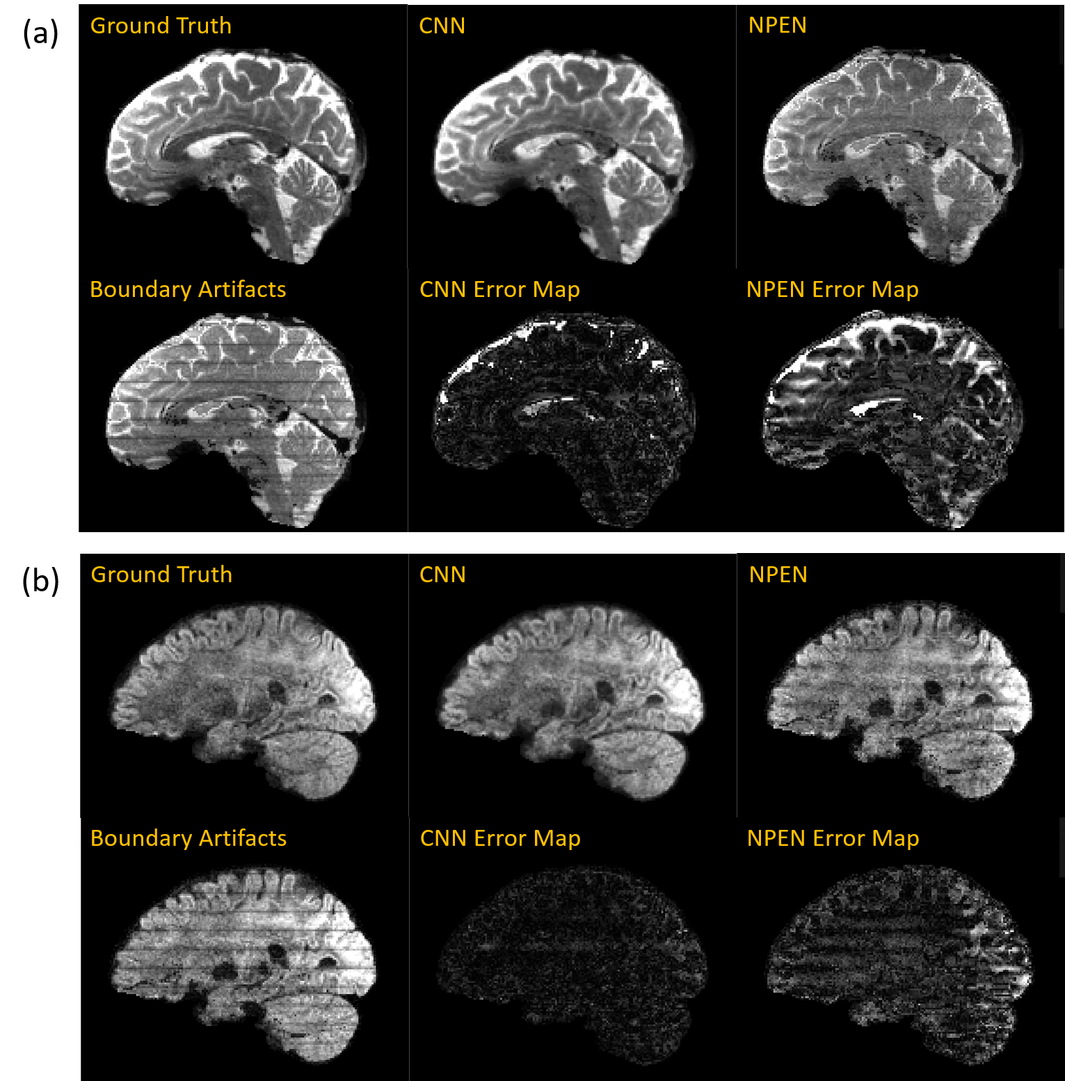
Fig.3 and Fig. 4 compare the results of the proposed method with NPEN. We can hardly see boundary artifacts in the images corrected by CNN, while residual artifacts are still visible in the results of NPEN. Moreover, CNN shows a strong suppression of noise, which provides a better vision of small fibers in the FA maps. NPEN has little resistance to noise, which leads to FA maps with low-quality.
Conclusion
From the results, we may draw a conclusion that the CNN-based method outperforms NPEN in boundary artifacts correction. It is noteworthy that the iterative NPEN method needs hours for computation of a whole-brain volume, which is impractical when a large amount of DWI volumes are acquired, while it takes a trained CNN model less than 1 second for it. Therefore, the CNN-based method is promising for boundary artifacts correction for the SMSlab acquisition. This study serves as a preliminary experiment for this idea. Ground truth data and real artifacts will be acquired for training in the next step.Acknowledgements
No acknowledgement found.References
1. Dai E, Wu Y, Wu W, et al. A 3D k-space Fourier encoding and reconstruction framework for simultaneous multi-slab acquisition. Magn Reson Med 2019;82(3):1012-1024.
2. Chen L FD. Simultaneous multi-slab echo volume imaging: comparison in sub-second fMRI. In Proceedings of the 21st Annual Meeting of ISMRM. Salt Lake City, 2013. p. 0303.
3. Wu WC, Koopmans PJ, Frost R, Miller KL. Reducing Slab Boundary Artifacts in Three-Dimensional Multislab Diffusion MRI Using Nonlinear Inversion for Slab Profile Encoding (NPEN). Magn Reson Med 2016;76(4):1183-1195.
4. Van AT, Aksoy M, Holdsworth SJ, Kopeinigg D, Vos SB, Bammer R. Slab Profile Encoding (PEN) for Minimizing Slab Boundary Artifact in Three-Dimensional Diffusion-Weighted Multislab Acquisition. Magn Reson Med 2015;73(2):605-613.
5. Engstrom M, Skare S. Diffusion-Weighted 3D Multislab Echo Planar Imaging for High Signal-to-Noise Ratio Efficiency and Isotropic Image Resolution. Magn Reson Med 2013;70(6):1507-1514.
6. Engstrom M, Martensson M, Avventi E, Skare S. On the Signal-to-Noise Ratio Efficiency and Slab-Banding Artifacts in Three-Dimensional Multislab Diffusion-Weighted Echo-Planar Imaging. Magn Reson Med 2015;73(2):718-725.
7. Parker DL, Yuan C, Blatter DD. MR angiography by multiple thin slab 3D acquisition. Magn Reson Med 1991;17(2):434-451.
8. Wu Yuhsuan DE, Yuan Chun, Guo Hua. Reducing slab boundary artifacts in 3D multi-band, multislab imaging. KSMRM. Seoul, 2018. p FA-086.
9. Jin KH, McCann MT, Froustey E, Unser M. Deep Convolutional Neural Network for Inverse Problems in Imaging. IEEE Trans Image Processing 2017;26(9):4509-4522.
10. Van Essen DC, Smith SM, Barch DM, et al. The WU-Minn human connectome project: an overview. Neuroimage 2013;80:62-79.
11. Jenkinson M, Beckmann CF, Behrens TEJ, Woolrich MW, Smith SM. FSL. NeuroImage 2012;62(2):782-790.
12. Ronneberger O, Fischer P, Brox T. U-Net: Convolutional Networks for Biomedical Image Segmentation. MICCAI. Cham, 2015.
13. Kingma DP, Ba J. Adam: A method for stochastic optimization. arXiv preprint arXiv:14126980 2014.
14. Wang Z, Bovik AC, Sheikh HR, Simoncelli EP. Image quality assessment: from error visibility to structural similarity. IEEE Trans Image Processing 2004;13(4):600-612.
Figures