Introduction

Diffusion weight imaging (DWI) often suffers low signal-to-noise ratio (SNR) at high b-values, which could introduce biases in quantitative analysis of DWI data. Although sum of square (SoS) coil combination scheme is widely used in MRI with phased array coils for optimal SNR, adaptive coil combine ¹ or SENSE1 ² are usually better solutions in diffusion MRI scans. If the SoS coil combine mode is mistakenly used, the amplified noise cannot be overcome by normal denoising techniques such as MPPCA ³. In this work, we investigated whether it is possible to use deep learning to reduce the SoS noise.

Methods

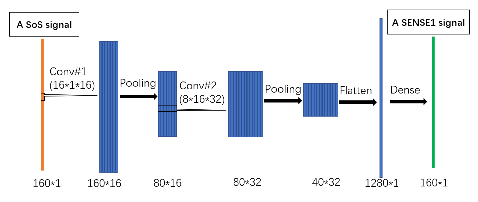
DWI data and processing: The DWI data of three subjects were acquired on a Prisma scanner using the HCP lifespan protocol: TR/TE = 3470/87 ms, 1.5 mm isotropic resolution, 37 gradient directions with b-value = 1000, 2500 s/mm² plus 6 b0 images, resulting a total of 80 images, SMS acceleration factor = 4. Each subject has two datasets with the same DWI protocol but with different coil combine modes: SoS and SENSE1. Each dataset consisted of data from two scan sessions with opposite phase encoding directions (AP and PA). For one subject, the two datasets were constructed from one scan and therefore used as training data. The datasets of the other two subjects were acquired from back-to-back scans and used as testing data. DWI data were processed in FSL for susceptibility distortion correction (TOPUP) and Eddy current/motion correction (using “eddy” command). Then tensor fitting was performed using weighted least square option to compute fractional anisotropy (FA) and mean diffusivity (MD). The neurite orientation dispersion and density imaging (NODDI) analysis ⁴ was performed using the NODDI Matlab toolbox (http://mig.cs.ucl.ac.uk/index.php). The intra-cellular volume fraction (ICVF) and orientation dispersion index (ODI) were obtained. The training data was used for deep learning by a convolutional neural network (CNN). The network learns denoising based on the voxel-wise SoS data (input) and SENSE1 data (target). The denoising model was then applied to the training data and two testing datasets for comparison.

Network structure: As a preliminary study, we constructed a simple model that has five layers, including two convolutional layers, each followed by a max-pooling layer, and a dense layer. The first convolutional layer takes the SoS DWI signals as input and has 16 one-dimensional filtering kernels of size 16. There are 32 filtering kernels of size 8 in the second convolutional layer. ReLU activation function is used in two convolutional layers. Both the two max-pooling layers have the kernel of size 2 with stride 2. The extracted features of the SoS DWI signals are finally mapped to the SENSE1 signals in the dense layer. The structure of the constructed model is shown in Fig. 1. The model was implemented in Tensorflow and python on a computer with 32 G memory, an AMD CPU and a Nvidia GPU. There were about 250,000 training samples, each with a length of 160 data points.

Results

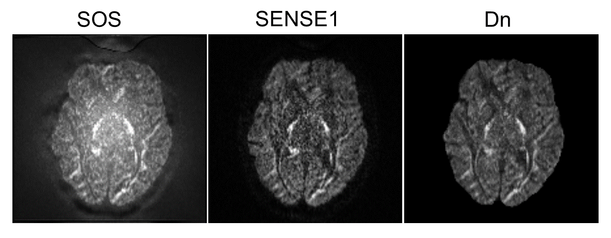
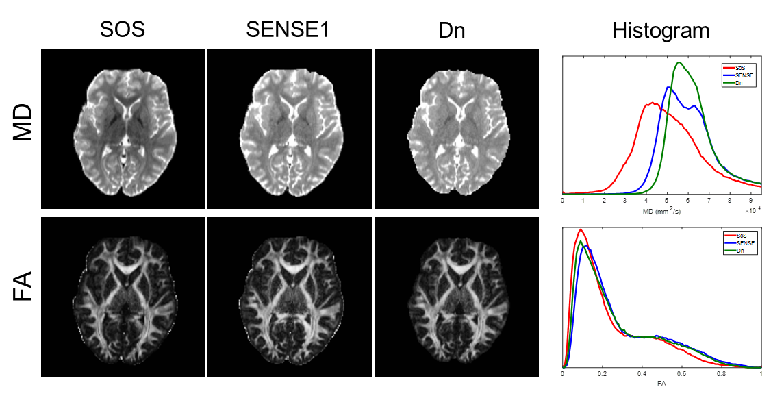
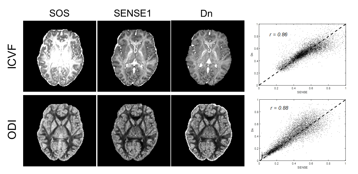
Fig. 2 compares SoS, SENSE1, and denoised images of b-value 2500 s/mm². The SoS image is higher in noise. The denoised (Dn) image is very similar to the SENSE image but more smoother.

The CNN model converged in 500 iterations within an hour. Fig. 3 shows an example of the FA and MD maps computed from SoS, SENSE1, and denoised data for testing subject 1, along with the histograms of FA and MD of the whole image volume. Both FA and MD are underestimated for SoS data. However, the underestimation is gone for FA in white matter in the denoised data although the MD might be slightly overestimated. Fig. 4 shows the ICVF and ODI map of SoS, SENSE1, and denoised data on the same slice of Fig. 3. There is apparent overestimation of ICVF and ODI for SoS data, with most white matter voxels having ICVF value equal to 1, which is due to abnormally high noise at high b-values (i.e., less signal attenuation). The ICVF and ODI maps are very similar for SENSE1 and Dn, as confirmed by the scatter plots. The correlation between the two is 0.86 for ICVF and 0.88 for ODI.

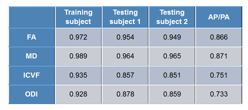
Table 1 lists the correlation coefficients of FA, MD, ICVF, and ODI between denoised and SENSE1 data for three subjects. It shows that the correlations are higher for the training subject, this is probably due to that the two datasets come from one scan and the testing is on the same subject of learning. The correlation of FA and MD is generally higher than that of ICVF and ODI. As a comparison, we also computed the correlation of these metrics between AP and PA SENSE1 data of testing subject 2. The correlations are much lower than those between SENSE1 and denoised.

Discussion

We have developed a simple deep learning method to retrospectively correct for SoS noise in DWI data. By acquiring two sets of diffusion images reconstructed with SoS and SENSE1 on one subject as training data, the learned model can effectively denoise any SoS data acquired with the same DWI protocol. This method also shed light on denoising techniques for diffusion imaging if a low-noise DWI dataset is available.

Acknowledgements

We thank CMRR of University of Minnesota for the multiband diffusion sequence. We thank Drs. Eddie Auerbach and Steen Moeller for their tremendous help in tracking down the noise problem and providing a solution to reconstruct both SoS and SENSE1 images.