0956
Diffusion phase-imaging using non-linear gradients in anisotropic synthetic fiber phantoms1School of Biomedical Engineering & Imaging Sciences, King's College London, London, United Kingdom, 2Philips Healthare, Guildford, United Kingdom, 3Department of Radiology, Massachusetts General Hospital, Athinoula A. Martinos Center for Biomedical Imaging, Charlestown, MA, United States, 4Inserm U1148, LVTS, University Paris Diderot, Paris, France
Synopsis
Diffusion MRI classically uses linear gradients to encode information about micro-structure in the loss of signal magnitude. When replaced by gradients varying quadratically in space, anisotropic diffusion results in a net phase shift, while the signal magnitude is largely preserved. This allows the extraction of information from signal phase inaccessible to other diffusion MRI methods. The phase evolution of anisotropic fiber phantoms were studied in simulations and diffusion experiments. Simulations confirm increasing phase change with increasing anisotropy and mixing time between diffusion gradients. First MR experiments with different mixing times show a phase shift in good agreement with theoretical estimate.
Introduction
Diffusion-weighted MRI uses the motion of water molecules to generate contrast. Usually, gradient fields varying linearly in space encode the diffusion of water in the signal magnitude. For large spin ensembles, diffusion is symmetric in space, i.e. an equal number of spins move in positive and negative direction. For linear gradients, this results in zero bulk phase change. The phase does not contain information about the probed tissue. Instead, spins within a voxel de-phase and signal magnitude drops.This changes with a quadratic gradient field. The presented method replaces the linear gradient with a quadratic Z2 field $$$ B_z=z^2-0.5(x^2 + y^2))$$$. In anisotropic media, diffusion in this gradient field results in a phase change. For isotropic diffusion, no phase shift is expected due to concomitant terms that ensure $$$\vec{B_z}=0 $$$. Around saddle point of the field $$$(x=y=z=0)$$$, there are no linear components that de-phase the signal. Therefore, a quadratic gradient encodes diffusion in signal phase while preserving large portions of the magnitude, thus improving SNR. Here, the phase evolution in fiber phantoms is investigated in Monte-Carlo simulations and MR experiments.Materilas and Methods
A theoretical concept was previously introduced [1] that allows predictions about the influence of a Z2 diffusion gradient on a spin ensemble. The expected change in net phase for 3D-diffusion is given by Equation(1)$$\varphi=-2\gamma\beta T(T+\Delta t)(D_z-0.5(D_x+D_y))$$
This expression assumes two identical (rectangular shaped) quadratic diffusion gradient pulses with curvature β, duration T, mixing time Δt.γ is the gyromagnetic ratio of water. $$$D_{x,y,z}$$$ are the diffusion coefficients in the corresponding directions. Equation(1) predicts a phase change only for anisotropic diffusion. To validate the theory numerically and experimentally, a collection of densely packed fibers are chosen as anisotropic medium since high fractional anisotropy (FA) is possible. Also, its well-known structure can be studied in simulations[2]. A numerical phantom was created in Camino[3] by generating randomly packed, impermeable cylinders. FA of simulated phantom is determined combining Equation(1) in with the simulated phase accumulations for multiple packing-densities. Based on [2], a phantom was manufactured with bundles of parallel synthetic Dyneema fibers, which were soaked in water and tightly packed in shrink tube. To avoid phase errors due to bulk motion, the phantom was placed in a glass tube with fomblin. A six-direction DTI-measurement (b-value=[0,2000]) using the scanner's linear gradients was performed to determine diffusivity and FA of the sample. Quadratic-gradient diffusion experiments on this phantom were carried out on a 3T Philips Achieva scanner with a custom-made coil insert (Figure1). Schematic and description of the 1DFT-STEAM-sequence can be found in Figure2(a). This sequence allows long mixing times Δt, repeated phase measurements in one image acquisition and also enables to acquire data with/without diffusion-weighting within same acquisition (Figure2(b)).The non-weighted data serves as reference to correct sequence-induced phase errors. Diffusion experiments are performed for diffusion pulse duration T=30ms, Δt1=600ms and Δt2=250ms, TR=3ms, TE=80ms. Also, MR-experiments with RF coil only were performed to characterize uncertainty of phase measurements.
Results
Simulations in fiber phantoms confirm a phase change for anisotropic diffusion. In accordance with the theory, Figure3(a) shows phase change increasing with FA. Phase change also increases with longer Δt (see Figure3(b)). DTI-measurement of the fiber phantom yields FA=0.6. The acquired magnitude and phase images for diffusion experiments with two Δt can be found in Figure4. In Figure5(a), error-bars for the phase measurements of the spatial position with highest signal magnitude are plotted. This point in space corresponds to the area around the saddle point of the Z2 field. The spread of phase measurements suggest that they are affected by noise. Noise analysis of the measured phase shows an error of 0.056rad (Δt1) and 0.048rad (Δt2). The phase data acquired in the RF coil only experiments have a standard error of 0.0035rad (error-bar in Figure5(b)). SNR for magnitude (SNR_Δt1= 13.5, SNR_Δt2=25.0) and phase (SNR_Δt1= 2.12, SNR_Δt2=8.86) were determined.Discussion and Conclusion
Diffusion MRI employing linear gradients to sensitize the signal magnitude to diffusion suffers from inherently poor SNR. The presented approach uses second order gradient fields to overcome these limitations by encoding (anisotropic) diffusion in the signal phase whilst preserving magnitude. Comparison of SNR shows a lower drop in SNR between Δt1 and Δt2 for phase than for magnitude data, although absolute value SNR is still higher for magnitude. This has to be addressed by reducing noise in phase acquisition (e.g. hardware improvements). Monte-Carlo simulations of fiber phantoms show a change in net phase dependent on the anisotropy of the sample as well as on experimental parameters, e.g. mixing time.MR data acquired with a custom made coil set-up show good signal for strong quadratic diffusion gradients and very long mixing times, both help, according to theory, to achieve a higher phase change. The measured phase difference of data acquired with two different Δt of 0.039 are in good agreement with the phase estimate provided by Equation(1) of 0.034rad. Higher uncertainty in diffusion measurements suggest additional noise is introduced when gradient coil is present and driven with current to generate gradient field. To reliably detect phase changes in this order of magnitude, the error on the phase measurements needs to be reduced, e.g. by acquiring more data points.Acknowledgements
This work is funded by the King’s College London & Imperial College London EPSRC Centre for Doctoral Training in Medical Imaging (EP/L015226/1) andPhilips Healthcare.References
[1] Wochner, Pamel, Stockmann, Jason, Schneider, Torben, Lee, Jack and Sinkus, Ralph. A novel approach to diffusion phase imaging using non-linear gradients in anisotropic media. Abstract 3499. ISMRM (2019), Montreal, CA.
[2] Fieremans, Els, et al. Simulation and experimental verification of the diffusion in an anisotropic fiber phantom. Journal of magnetic resonance 190.2 (2008): 189-199.
[3] P. A. Cook, Y. Bai, S. Nedjati-Gilani, K. K. Seunarine, M. G. Hall, G. J. Parker, D. C. Alexander, Camino: Open-Source Diffusion-MRI Reconstruction and Processing, 14th Scientific Meeting of the International Society for Magnetic Resonance in Medicine, Seattle, WA, USA, p. 2759, May 2006.
Figures
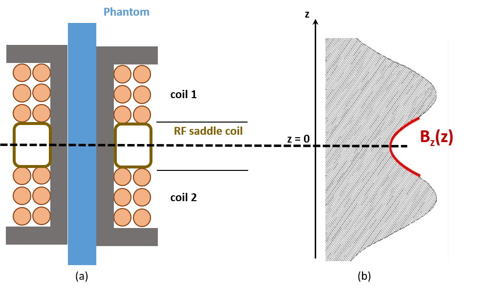
Figure1(a) Schematic coil insert. The Helmholtz pair consists of two coils with a length of 11 mm and 27 windings of 28 AWG insulated copper wire each. Inner diameter of the coil 10.5mm, outer diameter 12.5mm. The separation between coil 1 and coil 2 is 12mm. A RF saddle coil (transmit and receive) is fitted into the separation between the Helmholtz pair. No shielding.
(b) Gradient field Bz generated by Helmholtz coil along z-axis. Due to Maxwell’s equations the minimum along z-direction is in reality a saddle point. For the described coil design, β=23T/m2 is obtained for 1A coil current.
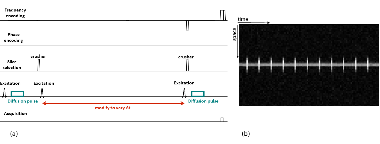
Figure2(a) 1DFT STEAM sequence. After first 90 degree excitation pulse, a diffusion gradient is applied. A second excitation pulse rotates net magnetization back into the longitudinal plane where it is stored and its net phase preserved. The spins are allowed to mix for the duration Δt before a third excitation pulse is followed by the second identical diffusion pulse. Δt is varied by varying time between second and third excitation pulse.
(b) Magnitude image acquired with 1DFT STEAM sequence. Interleaved lines with/without diffusion-weighting (every 8th line without as reference).
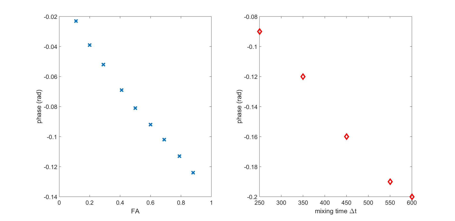
Figure3(a) Net phase plotted against different FA. Further simulation parameters were: pulse duration T=20ms, curvature β=25T/m2, Δt = 250ms.
(b) Net phase plotted over different mixing times Δt. FA = 0.6, other parameters as in above. The simulations confirm that confirm that the change in net phase increases with both increasing anisotropy of phantom and longer mixing time between diffusion gradient pulses.
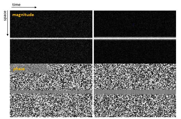
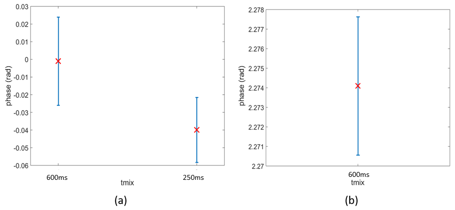
Figure5(a) Phase for two Δt was analyzed for pixel associated with saddle point of gradient field. Errors induced by sequence were corrected using reference data. Resulting phase error was determined using error propagation. Plot shows phase median (ensures outlier rejection) and error. A phase shift of 0.039 rad is observed between Δt1&Δt2. This shows good agreement with theoretical estimate (from Equation1)
(b) Error bar of phase acquired with RF coil only, no gradient coil present. 256 lines were acquired. Phase was analyzed for pixel associated with
position of saddle point.