Introduction

Microstructure sensitivity causes asymmetries in the bSSFP frequency response, in particular in white matter structures with distinct fiber tract orientations ^1,2. This substantially biases the relaxation time estimation based on conventional phase-cycled bSSFP relaxometry, such as MIRACLE ³ or PLANET ⁴. Recently, artificial neural networks (NN) proved the ability to learn gold standard brain tissue T₁ and T₂ values as well as robust field map estimates (transmit field B₁, off-resonance ∆B₀) from the asymmetric bSSFP frequency profile using a 12-point sampling scheme ⁵. Here, it is demonstrated that NN fitting is not only capable of providing accurate T₁ and T₂ values, but also shows promise to highly reduce the number of acquired phase-cycles while maintaining reasonable accuracy in the derived quantitative parameters.

Methods

For NN input, 3D sagittal bSSFP data was acquired at 3T (Prisma, Siemens Healthineers) in three healthy volunteers with 12 phase-cycles, evenly distributed in the range (0, 360°): φ_j = π/12∙(2j-1), j = 1,2,…12. The imaging was performed with an isotropic resolution of 1.3x1.3x1.3 mm³, 128 partitions providing whole brain coverage, a TR/TE of 4.8 ms/2.4 ms, α_nom = 15°, and a preparation block of 256 dummy pulses preceding each phase-cycle acquisition, leading to total acquisition time of 17 min 13 s using elliptical scanning. The NN training was applied to three different bSSFP sampling schemes: a 12-point scheme using all acquired phase-cycles φ_j (j = 1,2,…12), a 6-point scheme using every second acquired phase-cycle φ_2j-1 (j = 1,2,…6), and a 4-point scheme using only every third acquired phase-cycle φ_3j-1 (j = 1,2,…4). Voxelwise input into a 4-layer feedforward perceptron (3 hidden layers, 1 output layer) with 24 neurons in each hidden layer were the magnitude and phase of the Fourier transformed complex phase-cycled bSSFP data. Images were skull-stripped and voxels containing CSF were not included in the training. To prevent overfitting, Bayesian regularization was used as well as early stopping based on random division of the NN input data (~439’000 voxels) into training (70%), validation (15%), and testing (15%) subsets. Each N-point sampling scheme was trained for 10 different random initializations and the output was assessed as the average over all 10 networks.

To investigate the generalization performance on untrained data, an additional healthy volunteer was scanned using a 12-point, 6-point, and 4-point bSSFP phase-cycling scheme combined with in-plane GRAPPA acceleration 2 and otherwise identical parameters as described above, yielding acquisition times of 10 min 12 s, 5 min 6 s, and 3 min 24 s, respectively. For comparison, T₁ and T₂ maps were derived using conventional phase-cycled bSSFP relaxometry, here MIRACLE ³.

Target T₁, T₂, B₁, and ∆B₀ data for NN training and validation was acquired in all volunteers using dedicated reference methods. T₁: gold standard 2D multi-slice IR-SE with variable inversion times. T₂: gold standard 2D multi-slice single-echo SE with variable echo times. Total scan time for gold standard T₁ and T₂: 17 min 32 s / 30 slices, 2.6 mm slice thickness. B₁: TurboFLASH with and without preconditioning RF pulse ⁶. ∆B₀: standard dual-echo gradient-echo.

Results

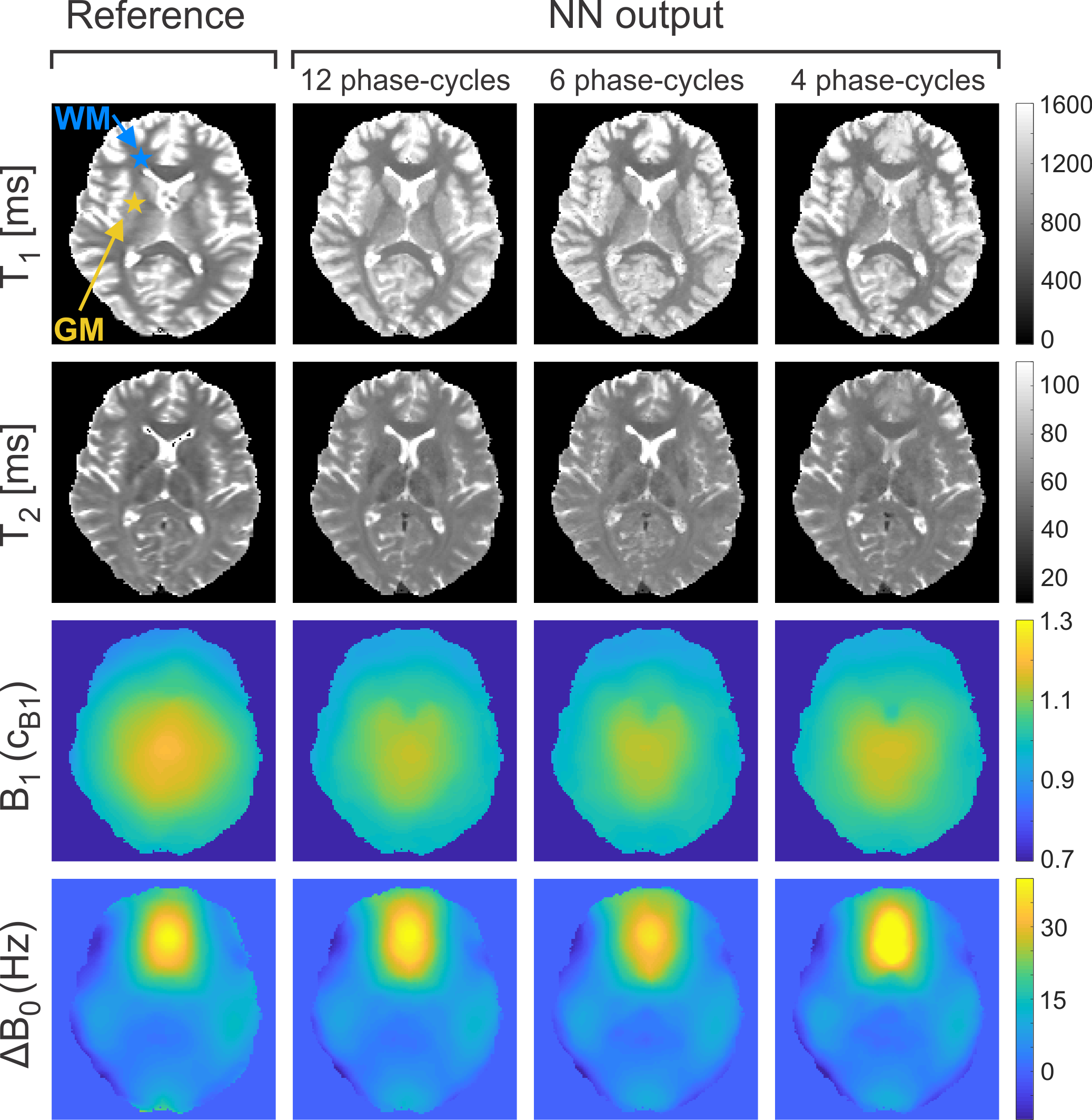
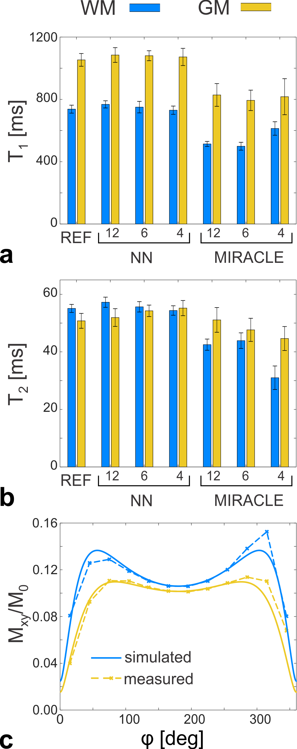
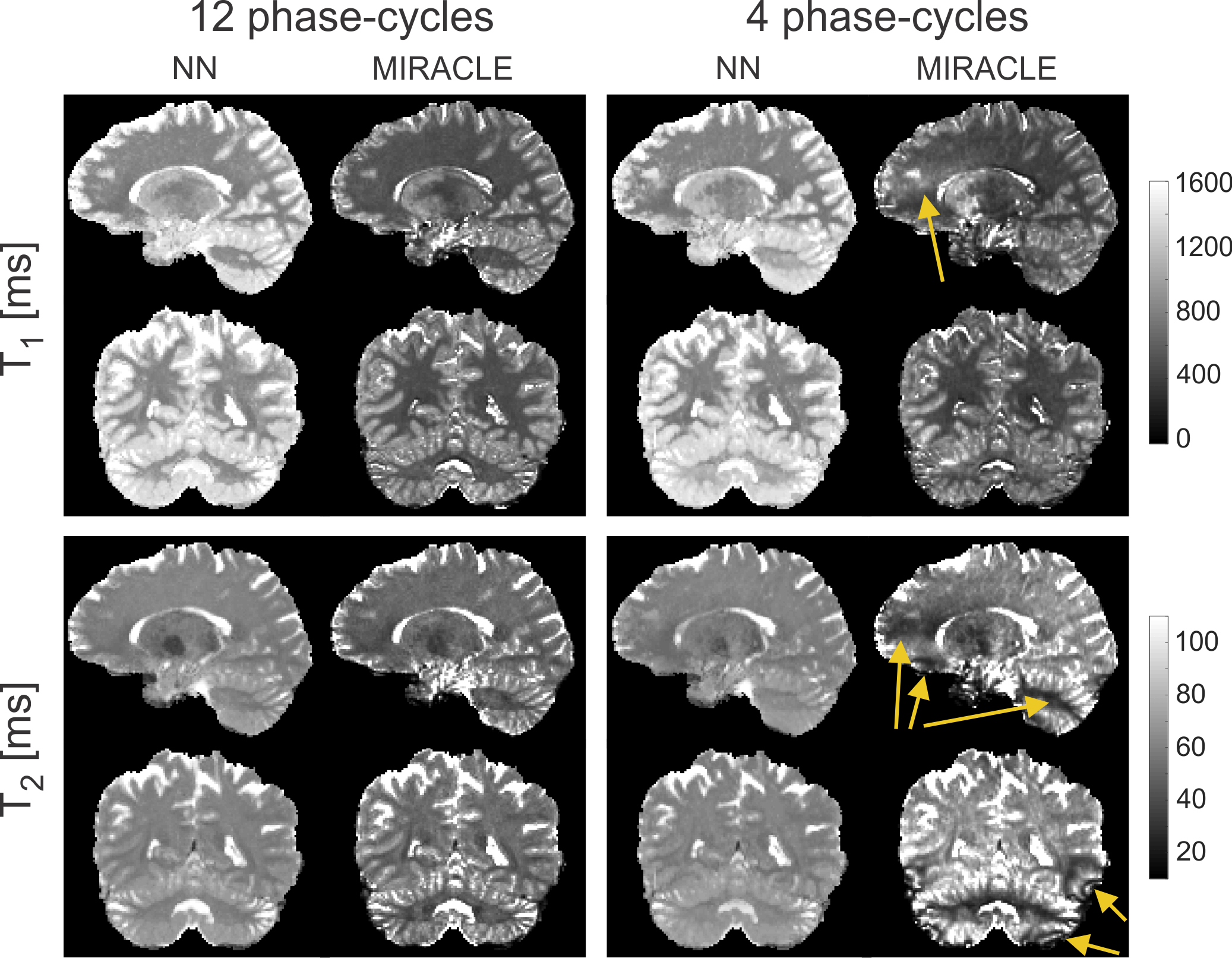
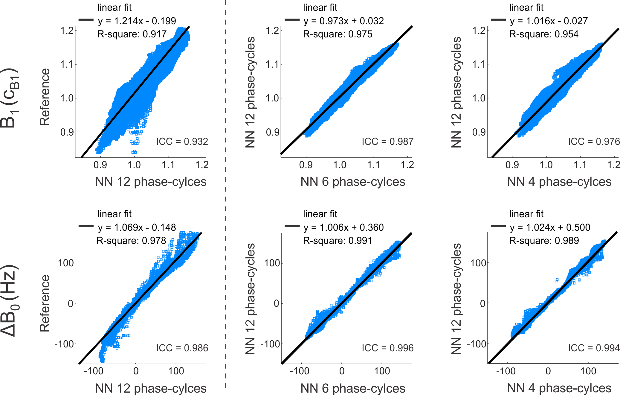
The NN prediction of relaxation times and field maps is shown in Figure 1 for a representative axial slice of untrained data in comparison to the reference measurements. Aside from a slight loss of contrast in the T₂ of deep gray matter (putamen), the 6-point and 4-point NN outputs demonstrate a high visual resemblance to the 12-point NN as well as to the reference data. In Figures 2a+b, the quantitative agreement of T₁ (Fig. 2a) and T₂ (Fig. 2b) with the gold standard is assessed for two representative ROIs located in white matter (frontal, blue asterisk in Fig. 1) and gray matter (putamen, yellow asterisk in Fig. 1). It can be observed that the NN maintains good agreement with the gold standard, even in case of only four acquired phase-cycles. In contrast, conventional phase-cycled bSSFP relaxometry (here MIRACLE) substantially underestimates T₁ and T₂ due to profile asymmetries (cf. Fig. 2c), and additional variability is introduced when the number of phase-cycles is reduced to four (Figs. 2a+b). Sagittal and coronal views of isotropic whole-brain T₁ and T₂ data derived from 12-point and 4-point NN fitting versus MIRACLE are displayed in Figure 3. The quality of 4-point MIRACLE T₁ and T₂ maps is clearly degraded and prone to off-resonance effects (cf. banding artifacts pointed out by yellow arrows in Fig. 3) while the NN fitting provides considerably more robust results. Whole-brain regression analysis of 12-point NN predicted B₁ and ∆B₀ maps of untrained data against reference data yields very good agreement between the two methods (cf. Fig. 4, left column). The correspondence of 6-point and 4-point versus 12-point NN B₁ as well as ∆B₀ values is remarkably high as reflected by intraclass correlation coefficients (ICCs) close to 1 (cf. Fig. 4, middle and right columns).

Discussion and Conclusion

NN fitting of phase-cycled bSSFP data has high potential to accelerate phase-cycled bSSFP relaxometry while simultaneously providing robust transmit and static field maps. A 4-point bSSFP phase-cycling scheme with an acquisition time of only 3 min 24 s allowed for rapid multi-parametric tissue characterization with whole-brain coverage at clinically relevant isotropic resolution.

Acknowledgements

No acknowledgement found.