Introduction

Subject motion is ubiquitous in clinical imaging and presents one of the major challenges for MR imaging of children as well as many other difficult patient populations. MR Fingerprinting (MRF) is a quantitative imaging technique which can provide simultaneous quantification of multiple tissue properties (1). Compared to conventional MR imaging, MRF often utilizes a non-Cartesian spiral trajectory for in-plane encoding, which is known to yield better performance in the presence of motion. The template matching algorithm used to extract quantitative tissue properties also provides a unique opportunity to reduce motion artifacts (1). However, with the prolonged 3D MRF acquisitions (typically around 5~10 min) (2-4), the scan is more susceptible to subject motions and further improvement in motion robustness is needed. In this study, we aimed to improve the motion sensitivity of 3D MRF technique by using fat navigator accelerated with spiral GRAPPA.

Methods

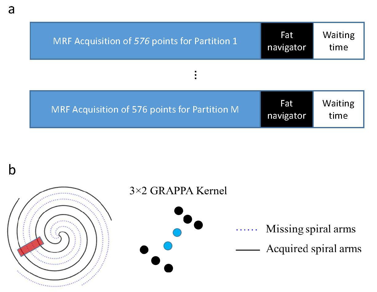
All measurements were performed on a Siemens 3T Skyra scanner using a 20-channel head coil. A 3D MRF protocol using variable flip angles and golden-angle spiral trajectories was adopted from the literature (5). The imaging parameters included: FOV, 30×30 cm; matrix size, 256×256; slice thickness, 3 mm; number of slices, 72; flip angles, 5°~12°; MRF time frame, 576. Similar to the original MRF method, each MRF time frame was highly undersampled in-plane by acquiring only one spiral arm (1). The partition direction is linearly encoded and acquired sequentially (Fig. 1a). A 2-sec waiting time was applied at the end of acquisition of each partition for longitudinal signal recovery. The total acquisition time for one 3D acquisition was about 11 min.

To improve the motion robustness of 3D MRF, a fat navigator (spatial resolution, 2×2×3 mm³) was inserted during the 2-sec waiting time at the end of each partition acquisition (Fig. 1a) (6). A 1-2-1 binomial RF pulse was used for fat excitation. Compared to previous implementation of a fat navigator at 7T, the chemical shift between fat and water is reduced from ~1000 Hz to 440 Hz at 3T, which increases the duration of the fat excitation pulses (~3.3 msec). To accelerate the 3D fat navigator to minimize the sensitivity of navigator itself to motion, a stack-of-spiral trajectory was used along with the spiral GRAPPA technique (Fig. 1b) (7,8). To identify the optimum setting for combined in-plane and through-plane accelerations, a 3D MRF scan was performed on a normal volunteer and the fat navigator was fully sampled during the scan. Retrospective undersampling was performed with various combination of in-plane and through-plane reduction factors and the results were compared to the reference results obtained with no acceleration.

We first validated the quantitative accuracy of the proposed method on phantom experiments and the results were compared to those acquired from the standard 3D MRF without the fat navigator. The proposed method was further tested on three normal volunteers (male; mean age, 48±9 years). The subjects were instructed to move intentionally during the MRF scans. Based on the reconstructed fat navigator images, motion signal was extracted using the SPM12 toolbox. Both translational and rotational motions were corrected in k-space followed by non-Cartesian imaging reconstruction. T1 and T2 maps were computed from 3D MRF datasets using pattern matching.

Results

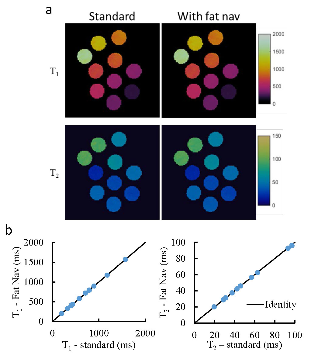
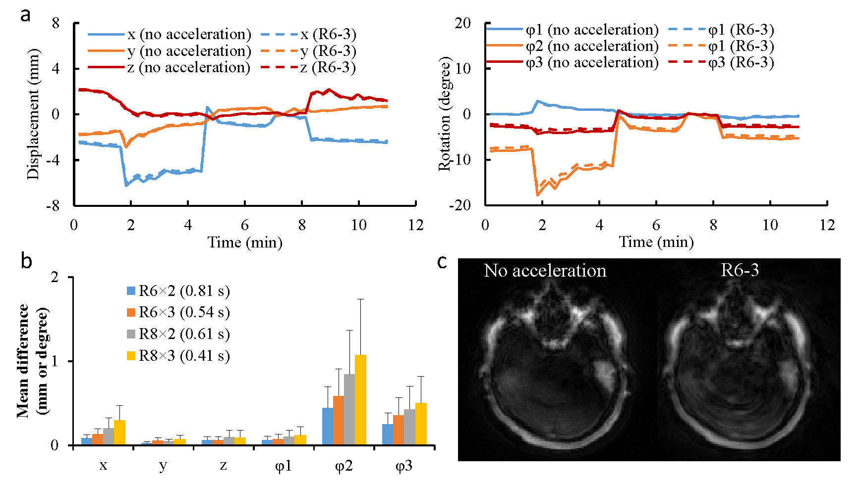
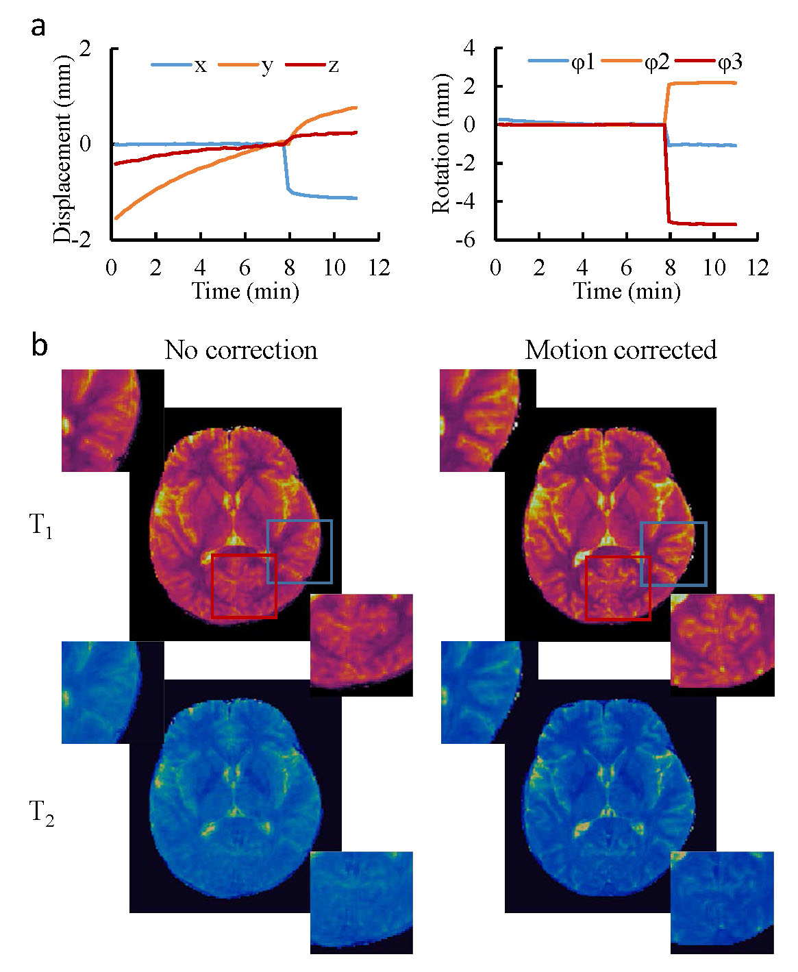
Fig. 2 shows the phantom results obtained with and without fat navigator. A good agreement was observed in both T1 and T2 values, which suggests that the application of fat navigator does not influence the tissue quantification based on water signal. Fig.3 shows the results of different acceleration schemes to acquire the fat navigator. A combined in-plane and through-plane acceleration of R6×3 was selected in the study based on the accuracy of motion tracking and the acquisition speed (~0.5 sec per navigator module). Representative T1 and T2 maps obtained with and without motion correction from a normal volunteer are presented in Fig. 4 along with the estimated motion curves. Fig. 5 shows an animation of T1 and T2 maps before and after motion correction from another volunteer. All these results demonstrate that the proposed method can be applied to effectively improve motion robustness for the 3D MRF method in neuroimaging.

Discussion and Conclusion

In this study, a fat navigator was integrated at each partition with 3D MRF to effectively reduce its motion sensitivity in neuroimaging. In combination with non-Cartesian spiral GRAPPA, a rapid fat navigator sampling (~0.5 sec) was achieved at 3T, reducing its sensitivity to potential motion. The improvement in motion robustness was achieved without increasing the scan time for quantitative tissue mapping. Since the current study was focused on evaluation of motion sensitivity of the proposed method, recent advances to accelerate 3D MRF itself were not applied (2-4). These methods can be combined with the proposed method to reduce the total acquisition time and motion artifacts in the future. Future studies will also be performed to evaluate its performance with various types of head motions, its accuracy for high-resolution quantitative imaging, and its application with challenging populations such as children.

Acknowledgements

No acknowledgement found.