0867
High Fidelity Direct-Contrast Synthesis from Magnetic Resonance Fingerprinting in Diagnostic Imaging1Electrical Engineering and Computer Sciences, University of California, Berkeley, Berkeley, CA, United States, 2Philips Research, Hamburg, Germany, 3Universitätsklinikum Bonn, Bonn, Germany, 4Bioengineering, UC Berkeley-UCSF, San Francisco, CA, United States, 5Electrical and Computer Engineering, The University of Texas at Austin, Austin, TX, United States, 6International Computer Science Institute, University of California, Berkeley, Berkeley, CA, United States
Synopsis
MR Fingerprinting is an emerging attractive candidate for multi-contrast imaging since it quickly generates reliable tissue parameter maps. However, contrast-weighted images generated from parameter maps often exhibit artifacts due to model and acquisition imperfections. Instead of direct modeling, we propose a supervised method to learn the mapping from MRF data directly to synthesized contrast-weighted images, i.e., direct contrast synthesis (DCS). In-vivo experiments on both volunteers and patients show substantial improvements of our proposed method over previous DCS method and methods that derive synthetic images from parameter maps.
Introduction
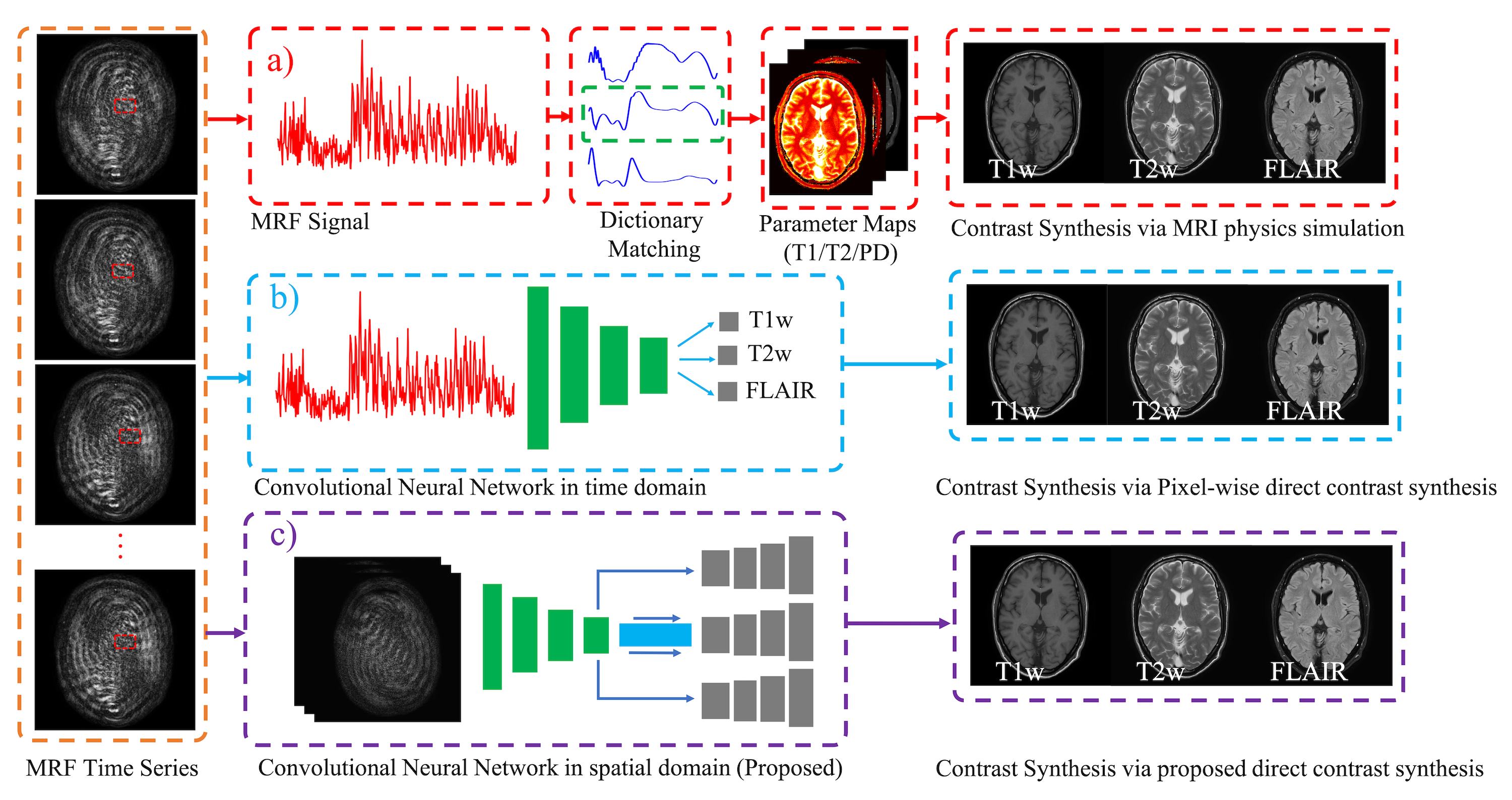
Multi-contrast images generated from a single scan have the tremendous potential to streamline and shorten overall exam times. Magnetic Resonance Fingerprinting (MRF) is an emerging attractive candidate for multi-contrast imaging since it has been shown to generate reliable quantitative tissue parameter maps1. Although tissue quantification can be useful for diagnosis, clinicians typically prefer qualitative, contrast-weighted images. With MRF, these images can be synthesized from the quantitative maps by simulating the MRI physics (e.g. Synthetic MR2). Unfortunately, contrast-weighted images generated from parameter maps often exhibit artifacts due to model imperfections (e.g. flow, partial voluming). To overcome these limitations, deep learning has recently been used to map acquisition data directly to contrast-weighted images3,4. One approach used a pixel-wise network to fit the MRF time series to a qualitative contrast weighting at each pixel3. However, the method did not leverage the spatial and structural information. Here, we propose a spatial-convolutional supervised method for direct contrast synthesis (DCS). We employ a Generative Adversarial Network (GAN)5 based framework, where MRF data can be used to synthesize T1-weighted, T2-weighted, and FLAIR images, which are common contrasts used in diagnostic imaging. Figure 1 summarizes the three different approaches of producing synthetic, multi-contrast images, out of which Figure 1.c is our proposed method. In-vivo experiments on both volunteers and patients show substantial improvements in image quality compared to previous DCS method and Synthetic MR from parameter maps.Methods
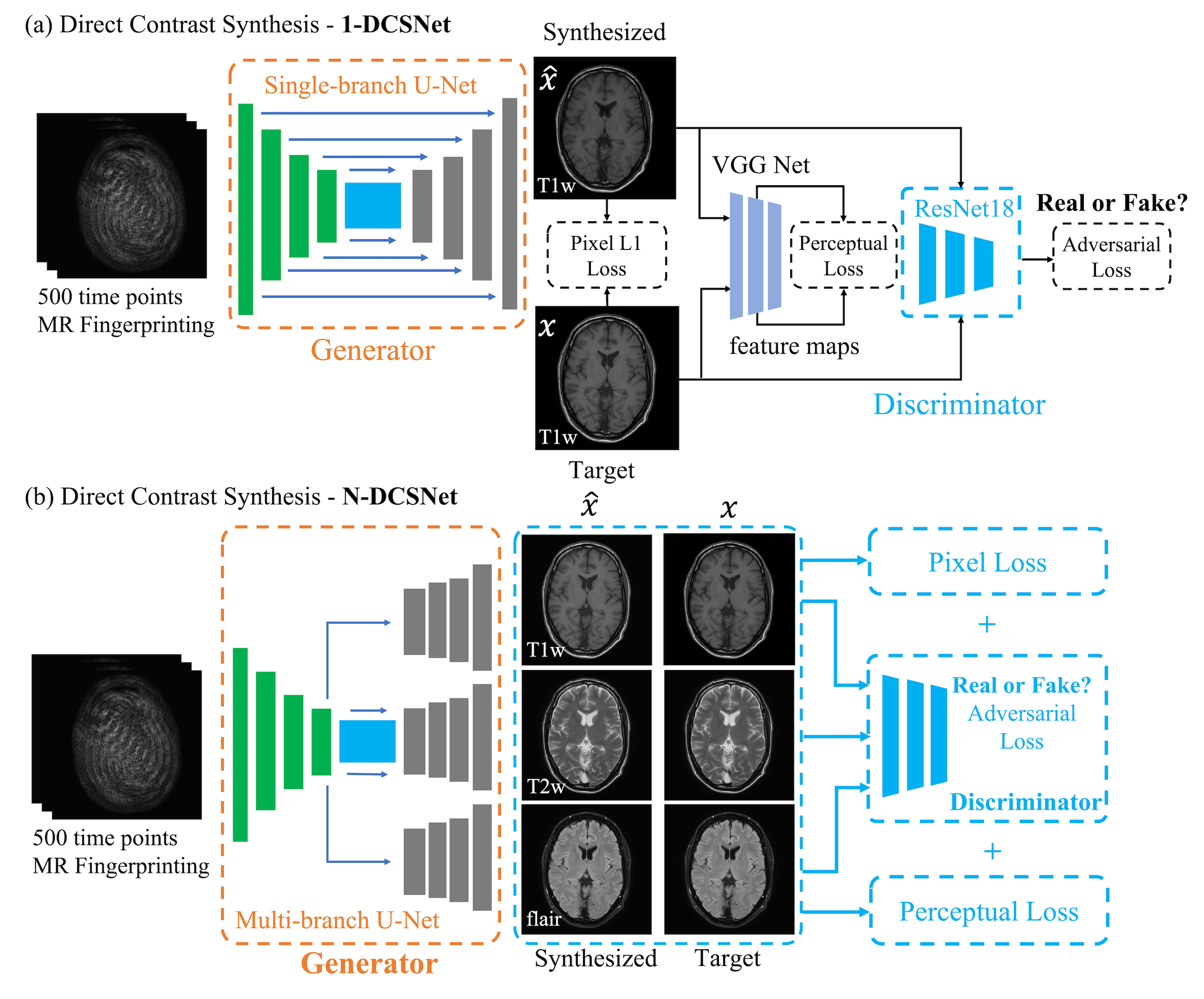
Network Design:We designed two GAN-based networks (1-DCSNet and N-DCSNet) for direct contrast synthesis from MRF data. Each network follows a standard conditional GAN framework with one generator $$$G$$$ and one discriminator $$$D$$$ (Figure 2). The generator is a U-Net7 based convolutional network, which consists of one encoder and a single (1-DCSNet) or multiple decoders (N-DCSNet), while the discriminator is a Residual Network8. The output of the discriminator predicts whether the images are real (ground truth) or fake (synthesized images). The N-DCSNet uses a joint encoder with independent decoders to synthesize multi-contrast images, with the idea that contrast images share mutual information. All of the networks are trained with the learning rates 0.0001/0.0005 (Generator/Discriminator) for 100 epochs with batch size 4.
Loss function:
As shown in Figure 2, the loss function is a combination of the $$$L_{pixel}$$$, the $$$l_1$$$ loss between the synthesized the ground truth images, adversarial loss $$$L_{adv}$$$, as determined by the discriminator, and the perceptual loss $$$L_{per}$$$, which is calculated as the $$$l_2$$$ loss between the feature maps outputted by pre-trained VGG Net9. Therefore, the total loss can be written as $$L_{total}=\lambda_1L_{pixel}+\lambda_2L_{per}+\lambda_3L_{adv},$$ where $$$\lambda_i,i=1,2,3$$$ are the weights for different losses. The addition of the adversarial and perceptual losses creates more realistic synthetic results. In order to make the training invariant to the input data scaling, we use a scaling invariant loss10, where we multiply a scalar $$$s$$$ to the output synthetic images $$$\hat{x}$$$ and use $$$s\hat{x}$$$ to compute the losses. $$$s$$$ is easily computed by solving a least square problem: $$\arg\min_s ||s\hat{x}-x||^2_2,$$ where $$$x$$$ is the ground truth image. All of the networks were implemented in Pytorch11 and trained using GeForce TITAN Xp GPUs.
Dataset and preprocessing:
All scans were performed with IRB approval and informed consent.
Volunteers: We scanned 21 volunteers between ages 29 to 61 years using a 1.5T Philips Ingenia scanner. 17 of the subjects were scanned twice, resulting in 38 datasets with 10 slices per sample. 36 samples are used as a training set while the other 2 are used as the test set.
Patients: A total of 30 patients (12 slices each) with different brain lesions (Parkinsons, Epilepsy, Tumor, Infarcts, etc.) were included in the study. All scans were conducted on a 3T Philips Achieva TX scanner. 26 out of 30 samples are used for training while the other 4 are used for testing.
For each sample in volunteers and patients, four MR examinations were conducted: T1w Spin Echo, T2w Turbo Spin Echo, FLAIR and a spiral MRF with variable flip angles (Captions in Figure 3 and 4 show the different sequence parameters for Volunteers and Patients). All the slices were normalized by the intensity of the white matter prior to training and testing. As the field strength and MRF parameters differed, separate networks were trained for the volunteers and patients' data.
Results
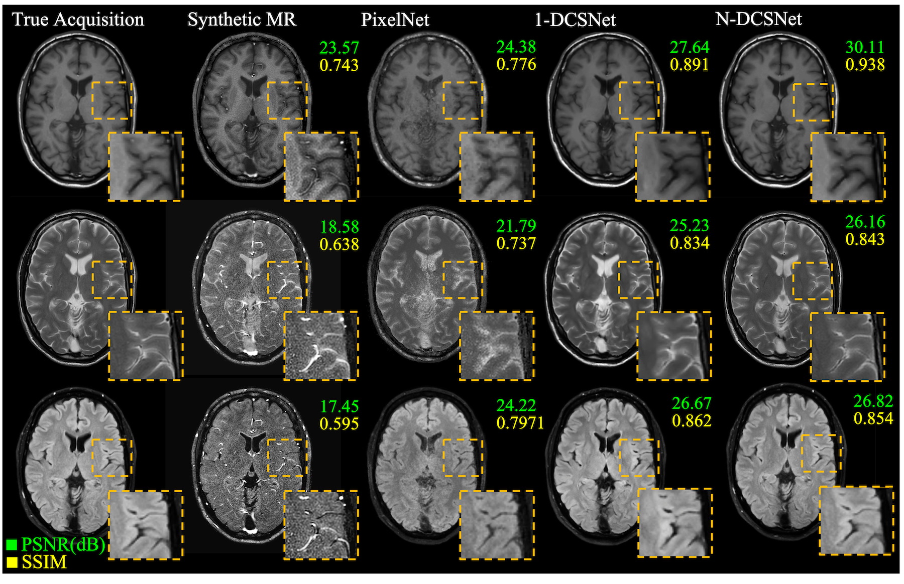
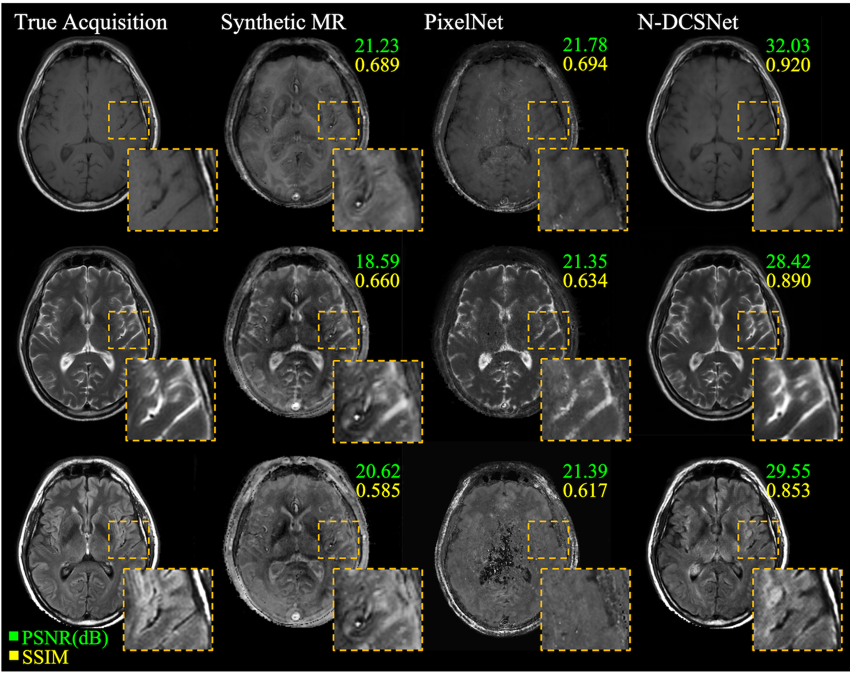
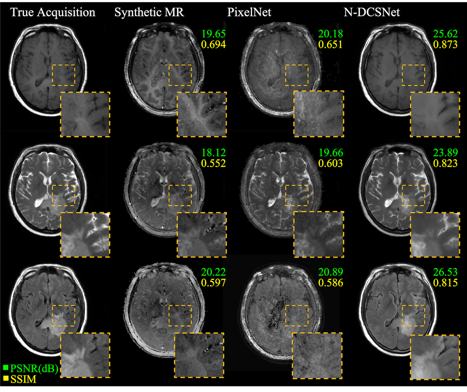
Figure 3 (Volunteers) and Figures 4 and 5 (Patients) display comparisons between different methods on three different synthesized contrasts in the test set. The high diagnostic quality of 1-DCSNet and N-DCSNet contrast images from MRF data is eminent, showing more structural details, higher peak signal-to-noise ratio (PSNR) and higher Structural Similarity Index (SSIM) compared to our implementation of PixelNet and Synthetic MR from parameter maps, even in the presence of large off-resonance artifacts.Discussion and Conclusion
Our proposed direct contrast synthesis method demonstrates that multi-contrast MR images can be synthesized from a single MRF acquisition with sharper contrast, minimal artifacts, and a high PSNR on both volunteers and patients. Additionally, N-DCSNet also implicitly learns some spiral deblurring. By directly training a network to generate contrast images from MRF, our method does not use any model-based simulation steps and therefore can also avoid any reconstruction errors due to simulation.Acknowledgements
No acknowledgement found.References
1. Ma, D., Gulani, V., Seiberlich, N., Liu, K., Sunshine, J. L., Duerk, J. L., & Griswold, M. A. (2013). Magnetic resonance fingerprinting. Nature, 495(7440), 187.
2. Hagiwara, A., Warntjes, M., Hori, M., Andica, C., Nakazawa, M., Kumamaru, K. K., ... & Aoki, S. (2017). SyMRI of the brain: rapid quantification of relaxation rates and proton density, with synthetic MRI, automatic brain segmentation, and myelin measurement. Investigative radiology, 52(10), 647.
3. Patrick Virtue, Mariya Doneva, Jonathan I. Tamir, Peter Koken, Stella X. Yu, and Michael Lustig.Direct contrast synthesis for magnetic resonance fingerprinting. In Proc. Intl. Soc. Mag. Reson. Med, 2018
4. Guanhua Wang, Enhao Gong, Suchandrima Banerjee, Huijun Chen, John Pauly, Greg Zaharchuk. OneforAll: Improving the Quality of Multi-contrast Synthesized MRI Using a Multi-Task Generative Model. In Proc. Intl. Soc. Mag. Reson. Med, 2019
5. Goodfellow, I., Pouget-Abadie, J., Mirza, M., Xu, B., Warde-Farley, D., Ozair, S., ... & Bengio, Y. (2014). Generative adversarial nets. In Advances in neural information processing systems (pp. 2672-2680).
6. Hennig, J., Weigel, M., & Scheffler, K. (2004). Calculation of flip angles for echo trains with predefined amplitudes with the extended phase graph (EPG)‐algorithm: principles and applications to hyperecho and TRAPS sequences. Magnetic Resonance in Medicine: An Official Journal of the International Society for Magnetic Resonance in Medicine, 51(1), 68-80.
7. Ronneberger, O., Fischer, P., & Brox, T. (2015, October). U-net: Convolutional networks for biomedical image segmentation. In International Conference on Medical image computing and computer-assisted intervention (pp. 234-241). Springer, Cham.
8. He, K., Zhang, X., Ren, S., & Sun, J. (2016). Deep residual learning for image recognition. In Proceedings of the IEEE conference on computer vision and pattern recognition (pp. 770-778).
9. Simonyan, K., & Zisserman, A. (2014). Very deep convolutional networks for large-scale image recognition. arXiv preprint arXiv:1409.1556.
10. Eigen, D., & Fergus, R. (2015). Predicting depth, surface normals and semantic labels with a common multi-scale convolutional architecture. In Proceedings of the IEEE international conference on computer vision (pp. 2650-2658).
11. Paszke, A., Gross, S., Chintala, S., Chanan, G., Yang, E., DeVito, Z., ... & Lerer, A. (2017). Automatic differentiation in pytorch.
Figures