Introduction

Prostate cancer (PCa) is the second most frequently diagnosed cancer in men (1). Multi-parametric MRI (mp-MRI) is increasingly used for PCa detection and staging. There has been a growing interest in applying deep learning techniques such as convolutional neural networks (CNN) to radiological images (2), including prostate mp-MRI (3-5). We have developed a novel CNN architecture and combined it with advanced techniques (transfer learning, unsupervised pre-training, and test-time augmentation) to perform dense prediction (pixel by pixel classification of cancer vs. non-cancer). We used logistic regression (LR) and random forest (RF) as baseline models to judge the overall performance of the CNN model.

Methods: MRI and histopathological correlation

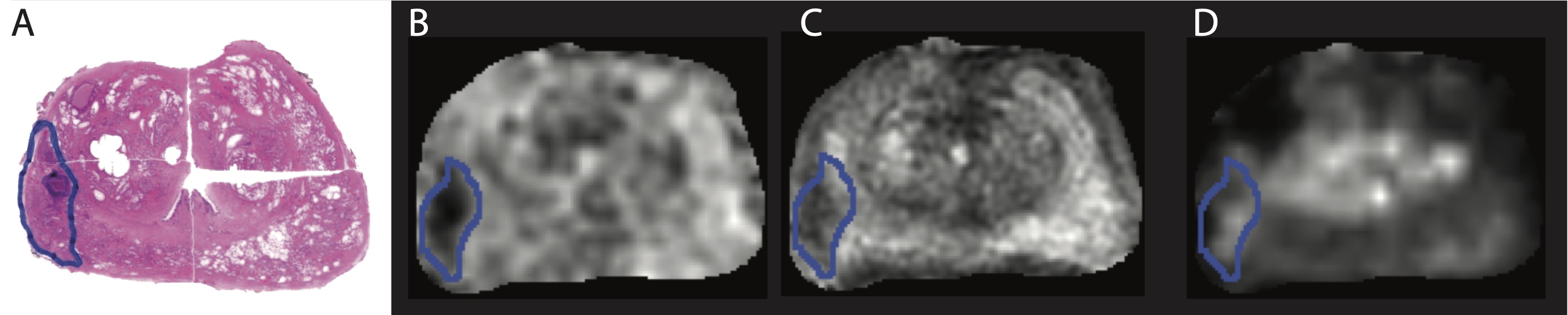
Approval was granted by the institutional Research Ethics Board. 154 patients referred for clinically indicated mp-MRI were prospectively recruited. Nineteen of these subjects subsequently underwent radical prostatectomy; of these, 3 subjects were excluded for motion artifact (n=1) and insufficient data to calculate a ktrans map (n=2), leaving 16 subjects with both mp-MRI and histopathological correlation. Subjects were scanned on a 3T MR750 (General Electric Healthcare, Milwaukee, WI, USA) with a 32-channel cardiac phased array receive coil (Invivo Corp, Gainesville, FL, USA) Sequence parameters can be found in (6). A fellowship-trained abdominal radiologist correlated the histopathological sections and/or the final pathology report with the mp-MR images and manually delineated the tumour margins on either T2w or ADC maps according to PIRADS 2 (7) (Figure 1).

Methods: Data Analysis

Model evaluation
Models were evaluated using F1 score, area under the precision-recall curve (AUPRC) and area under the receiver operating curve (AUROC) with leave-one-subject-out cross validation. Statistical significance (p<0.05) was determined using the paired Wilcoxon signed rank test with Benjamini-Hochberg correction for multiple comparisons.

Logistic Regression and Random Forest
Our implementation of LR was parametrically simple as no interaction terms were included. We mitigated the effects of class imbalance by modifying the class weights. For each leave-one-subject-out cross validation instance, we trained the LR model with different class weights in the range of [0.01, 0.99]. We selected the weight that achieved the best F1-score for the training subjects as the weight used to evaluate the test subject.The RF model was implemented using the scikit-learn machine learning library for Python (8). The model had 20 estimators (decision trees) and a maximum depth of 6. Gini impurity was used as the split criterion for the random forest. Class weights were applied and chosen using the same procedure as LR.

CNN Implementation
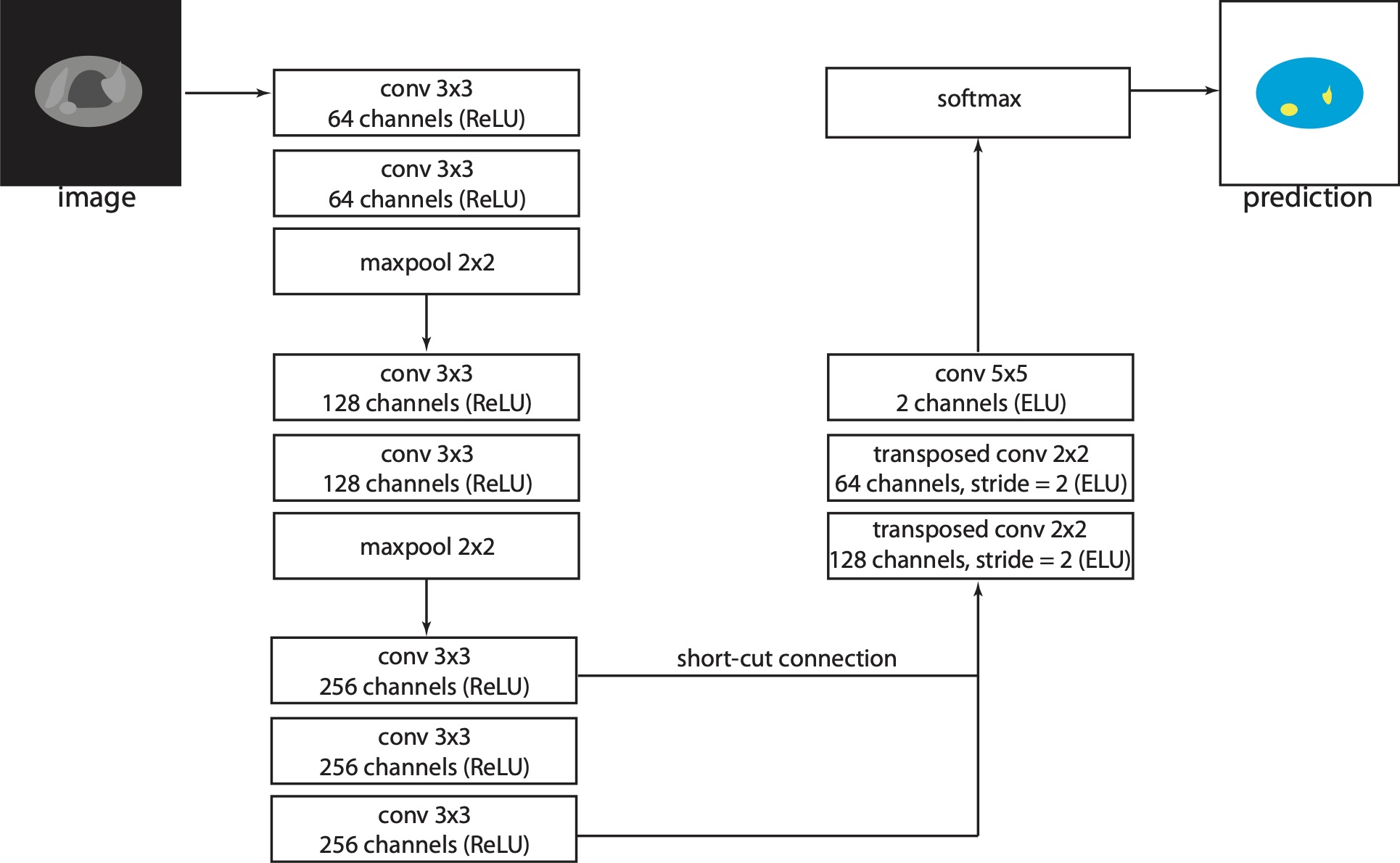
The architecture proposed in this work is a modification of VGG D net (9) (figure 2). The software for training and testing the CNN was written in Python and implemented using Tensorflow (10). We investigated whether the performance of the CNN model could be further improved by exploring transfer learning, unsupervised pre-training and test-time augmentation.

Transfer learning
We did not pre-train the network from scratch, but instead downloaded the pre-trained weight parameters (http://www.cs.toronto.edu/ frossard/post/vgg16/). The benefit of this approach was that we did not need to randomly initiate the weights for the lower layers of the network but could exploit the low-level features and filters already learned using the ImageNet dataset.

Unsupervised pre-training
Unsupervised pre-training is effective for improving the robustness of deep networks (11). The dataset consisted of mp-MRIs from the 135 consented subjects who did not undergo prostatectomy. Each image, before being processed by the network, was copied and then modified by randomly setting the value of some image pixels to zero. The modified image was used as input for the CNN while the original image was used as the labeled output; the network was therefore tasked with reconstructing the original pixel intensities. The cost function was the mean squared error between the network’s output and the original image pixel intensities.

Test-time augmentation
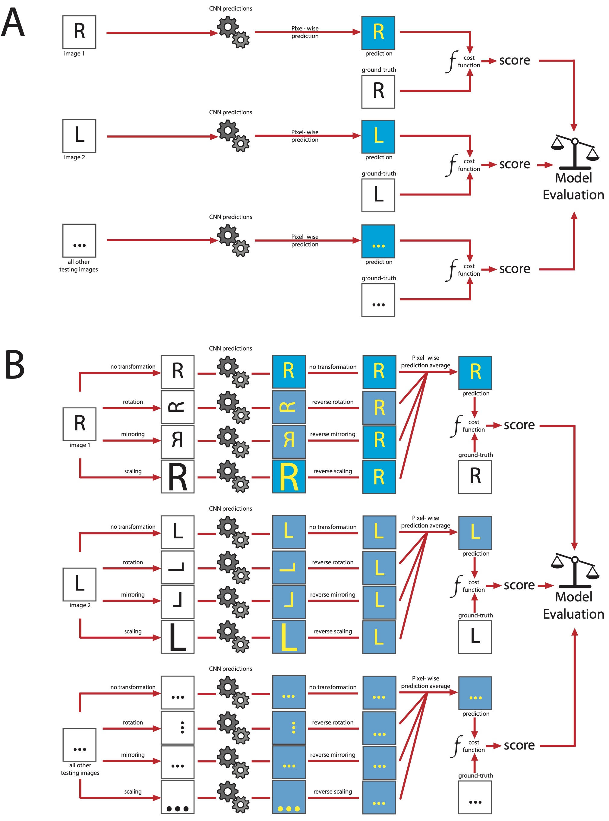
Test-time augmentation is a post-processing technique performed during the testing phase (12). After the network has been trained and the parameters optimized, each image in the test dataset goes through a series of transformations; in this case, scaling (scaling parameter range: 0.9 to 1.0), rotation (angle range: 6.0 to -6.0) and flipping (sagittal plane only). Each modified image, as well as one copy of the original image, were processed by the network which computed its prediction task. The predicted output was rectified by undergoing the inverse of the transformation. Finally, the multiple predictions were averaged (figure 3).

Results

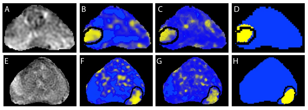
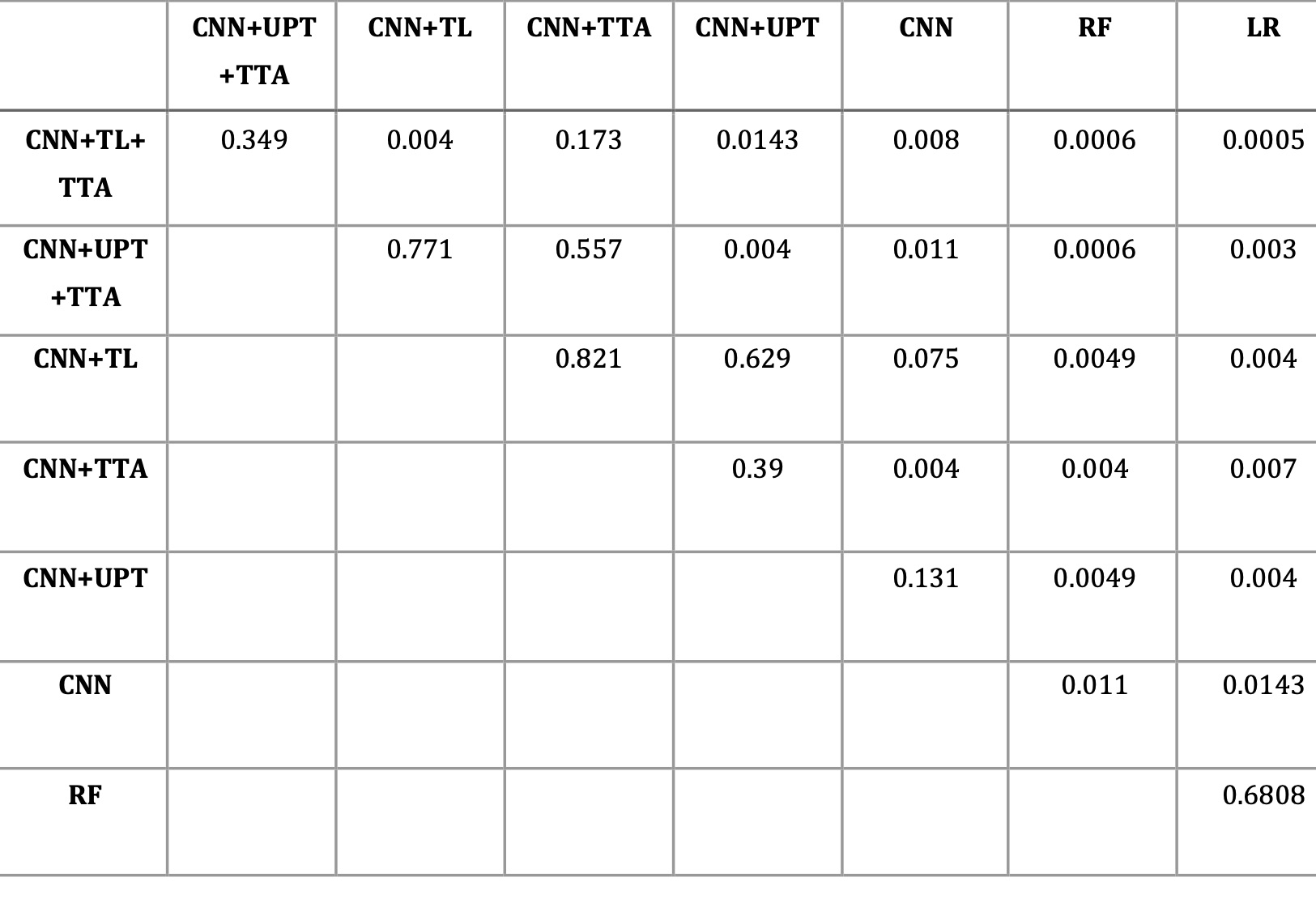
Baseline CNN outperformed logistic regression and random forest models. Transfer learning and unsupervised pre-training did not significantly improve CNN performance; however, test-time augmentation resulted in significantly higher F1 scores over both baseline CNN and CNN plus either of transfer learning or unsupervised pre-training (figure 4). The best performing model was CNN with transfer learning and test-time augmentation (F1 score of 0.59, AUPRC of 0.61 and AUROC of 0.93). Comparison between models is shown in table 2.

Conclusion

We have identified a novel CNN architecture that, in combination test-time augmentation with transfer learning or unsupervised pre-training, performs well on semantic segmentation of prostate cancer from mp-MRI examinations. The CNN model described statistically outperforms RF and LR baseline models even in a small dataset.

Acknowledgements

This work is supported by the Atlantic Innovation Fund, an Investigator Sponsored Research Agreement with GE Healthcare, Brain Canada, the Radiology Research Foundation, Canada Summer Jobs Program, Nova Scotia Cooperative Education Incentive grant and Google Cloud. The authors would like to acknowledge Liette Connor for help with recruitment, Manjari Murthy, Jessica Leudi, Nathan Murtha and Allister Mason for consenting participants and David McAllindon for creating the pseudo-wholemount histopathology sections.