Introduction

Image-guided radiotherapy using a hybrid MRI linear accelerator (MR-linac) system could enable compensation of breathing-induced motion by updating the multileaf-collimator with respect to tumor position. This requires an accurate measure of tumor position, derived from the MR data. Such adaption is never instantaneous but is delayed by latencies between 300ms and 436ms on the MR-linac¹, leading to increased error margins during planning. This margin could be reduced through an extrapolation of future tumor positions.
Recurrent neural networks (RNNs) proved to be useful for sequential tasks such as breathing motion prediction². Their structure allows them to incorporate their own history into the next prediction. In this study, the possibility of 1D motion predictions of the diaphragm up to latencies of 400ms on a MR-linac using a long short-term memory³ (LSTM) RNN was investigated.

Methods

Implementation
The LSTM network (Fig1A) was implemented using PyTorch-1.0.0. It consisted of a linear input/output layer and several hidden LSTM layers. The LSTM-units were initialized with cell- and hidden-states of zero.
The input to the network were phase data around the k-space center from multiple 1D k-space projections, updated at 10Hz in a sliding-window fashion. The network output were motion predictions at increments from 100 to 400ms into the future. The LSTM network was validated in simulations, a phantom experiment and finally demonstrated in vivo.

Simulations
Images consisting of a single line were generated, and the line was subjected to a 1D translation according to a sin⁴-function with amplitudes between 5-15mm and cycles between 1.58-2.5s (Fig1B). A 1D-Fourier-Transform was applied at each time step to simulate a 1D projection.

Phantom and in vivo
A motion phantom (Fig1C, constructed in-house⁴, MR-compatible motor from CIRS Inc., Norfolk, Virginia, USA) was driven with 21 different frequency and amplitude combinations of sin⁴-waves, distributed manually over an amplitude range of 5-10mm and cycles between 1.5-5s.
One healthy subject was measured in order to predict diaphragm position and was guided to breathe either “deep” or “normal”.
For both, phantom and subject, 1D-projections were taken in the Head-Foot direction from a bSSFP-sequence⁵ with TR=10ms. The projections were acquired on a 0.35T MRIdian-Linac system (ViewRay Inc., Cleveland, Ohio, USA) using two 6-channel body receive coils with Δx=1.17mm.
After offline reconstruction, the motion was extracted by comparing the first image of each dataset to following frames in the region of interest. The base frame was rigidly shifted until the mean squared difference of both frames was minimized. Based on these shifts, the motion was reconstructed.

All data was cut into approximately 8s long time series and 10 independent models were trained. The models were tested on data withheld during training of approximately 10%-20% of the training set size. During training, the mean-squared-error (MSE) between the prediction $$$\hat{y}$$$ and ground-truth $$$y$$$ was minimized over all N examples using Adam⁶. The resolution is given as the root-mean-squared-error (RMSE):
$$\mathrm{RMSE}=\sqrt{\Sigma_{n=1}^{N}(\hat{y}-y)^2}$$

Results

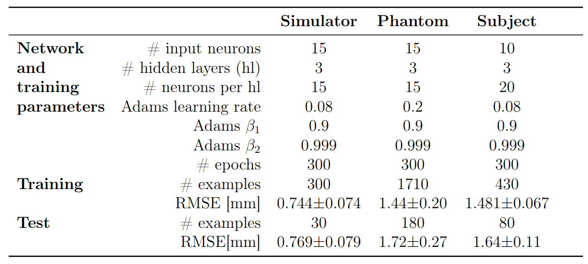
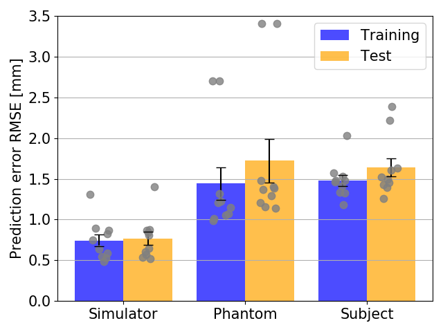
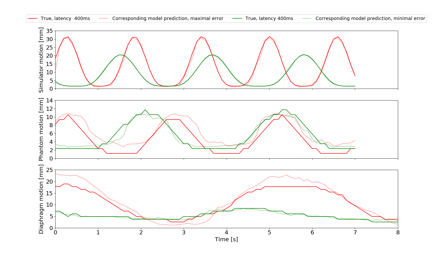
The network configurations for each experiment and respective performance results are shown in Figures 2 and 3.
The best models for each motion type were compared, with Figs4A-C showing the best and worst prediction performances. The RMSE for the diaphragm ranged from 0.410mm/0.45mm to 4.419mm/2.35mm (train/test).
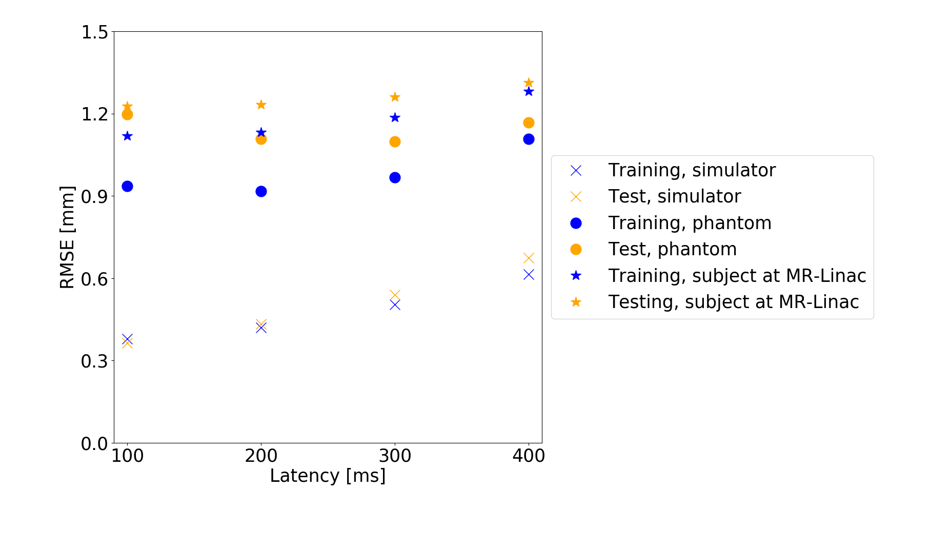
Fig5 shows the average prediction performance for latencies 100-400ms.

Discussion

The simulations outperformed the MRI-measurements because training and test set are randomly sampled from the same data distribution and are not subject to noise.
There was larger model-to-model performance variation for the phantom. This may be due to a suboptimal network structure less robust to variations in initial conditions. The larger learning rate contributes to this effect by allowing the system to possibly jump out of minima instead of converging into them.
However, in vivo diaphragm motion was successfully predicted from 1D-projections with a precision of approximately 1.7mm up to a 400ms latency. At certain examples, an increased RMSE in the motion predictions was observed (Fig3C). It is likely, that motion occurred on which the LSTM network had not been trained intensively compared to others. Words such as „deep“ or „normal“ are subjective and need a more sophisticated acquisition protocol. Fast switching between the states can lead to less stable breathing patterns. If there is relatively few data on switching compared to long single state acquisitions, the training set is unbalanced and the network fails to predict the less stable patterns. The network is then overfitted.
The number of inputs for the in vivo experiment was reduced to increase prediction accuracy. It is likely, that smaller time windows are favorable for less consistent motion cycles such as breathing.
Each network was trained on an average error across all latencies, hence they show similar prediction accuracies. However, larger latencies are more difficult to predict.

Conclusion

The study showed the feasibility of predicting diaphragm motion based on MR k-space data using LSTM networks. This could allow for the real-time tracking and prediction of breathing induced motion.
The simultaneous prediction of motion between 100 to 400ms can be advantageous to compensate for dead times due to collimator adjustments during tracking-based treatment⁷. Future work will be focused exploring 2D motion prediction, optimizing the training and evaluation routine and the comparison between LSTM and other networks.

Acknowledgements

No acknowledgement found.