0771
Cardiac Tag Tracking with Deep Learning Trained with Comprehensive Synthetic Data Generation1Radiology, Stanford, Palo Alto, CA, United States, 2Mechanical Engineering, University of Central Florida, Orlando, FL, United States, 3Radiology, Veterans Administration Health Care System, Palo Alto, CA, United States, 4Cardiovascular Institute, Stanford, Palo Alto, CA, United States, 5Center for Artificial Intelligence in Medicine & Imaging, Stanford, Palo Alto, CA, United States
Synopsis
A convolutional neural network based tag tracking method for cardiac grid-tagged data was developed and validated. An extensive synthetic data simulator was created to generate large amounts of training data from natural images with analytically known ground-truth motion. The method was validated using both a digital cardiac deforming phantom and tested using in vivo data. Very good agreement was seen in tag locations (<1.0mm) and calculated strain measures (<0.02 midwall Ecc)
Introduction
Cardiac MRI (CMR) tagging enables the quantitative characterization of global (e.g., torsion) and regional cardiac function (e.g., strain), but its clinical adoption has long been hampered by painful post-processing methods. Despite the challenge of extracting the information, these quantitative measurements are important for understanding cardiac dysfunction, evaluating disease progression, and characterizing the response to therapy.Numerous methods for tracking tags exist [1-4]. However, many include laborious segmentation and tag-tracking corrections, or other substantial user input. Convolution neural networks (CNN) are well suited to both imaging segmentation [5] and motion tracking [6]. Training a CNN, however, requires: 1) a large amount of training data; and 2) the associated ‘ground truth’ tag motion. Herein, a CNN approach was developed for fast and automatic tag tracking. To properly train the network, we used an extensive data generation and simulation framework. The approach generates a large amount of synthetically tagged data from natural images combined with programmed tag motion and a full Bloch simulation. These images are then used to train a neural network to generate grid tag motion paths from the input images.
Methods
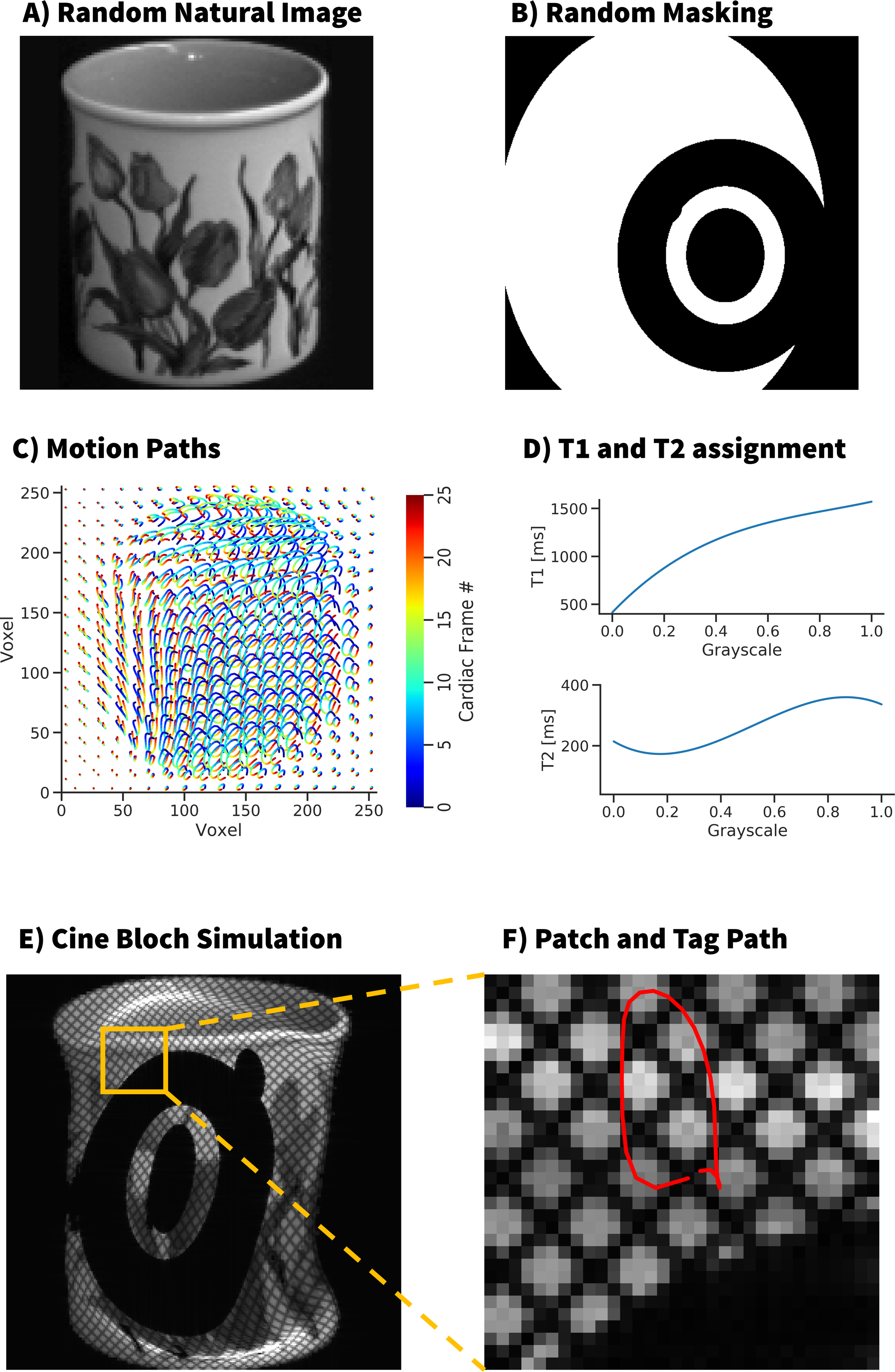
Synthesis of Motion Field Training ImagesImages were randomly selected from a database of natural images (Fig 1A). Random annular masks (Fig 1B), and periodic motion fields were applied (Fig 1C). The motion fields were generated with a set of randomly generated parameters describing an ellipse shape, as well as an additional 2nd order polynomial on the x and y positions of the path. T1 and T2 values were also randomly assigned by mapping grayscale values on a 3rd order polynomial with random parameters (Fig 1D). These dynamic training images were used as the input to a Bloch simulation that generated tagged images of the moving objects (Fig 1E). The simulation added complex gaussian noise (SNR=10-50), and grid tag spacing = 4-12 mm, and a 256x256 image matrix with 25 timeframes. The images were cropped to a 32x32 voxel patch dataset with 25 timeframes, centered around the tag location to be tracked at t=0. The analytic ‘ground truth’ tag motion paths were used for training (Fig 1F).
Computational Cardiac Phantom
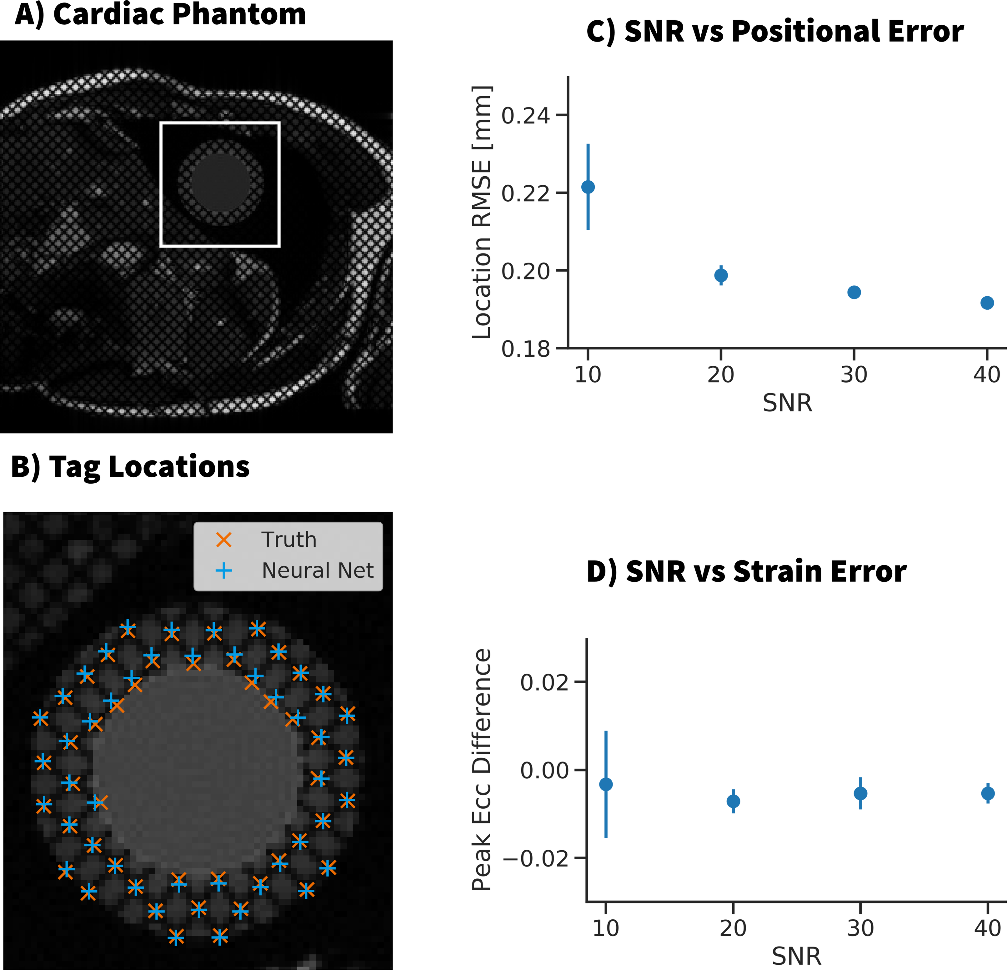
The trained network was tested on synthetic cardiac MR images generated using a computational deforming cardiac phantom [7] (Fig 3A). The trained CNN was compared to both the ‘ground truth’ tag locations and strain values. The performance was measured for a range of SNR values by comparing RMSE of the tag locations and the error in peak midwall circumferential strain (Ecc).
In Vivo Data
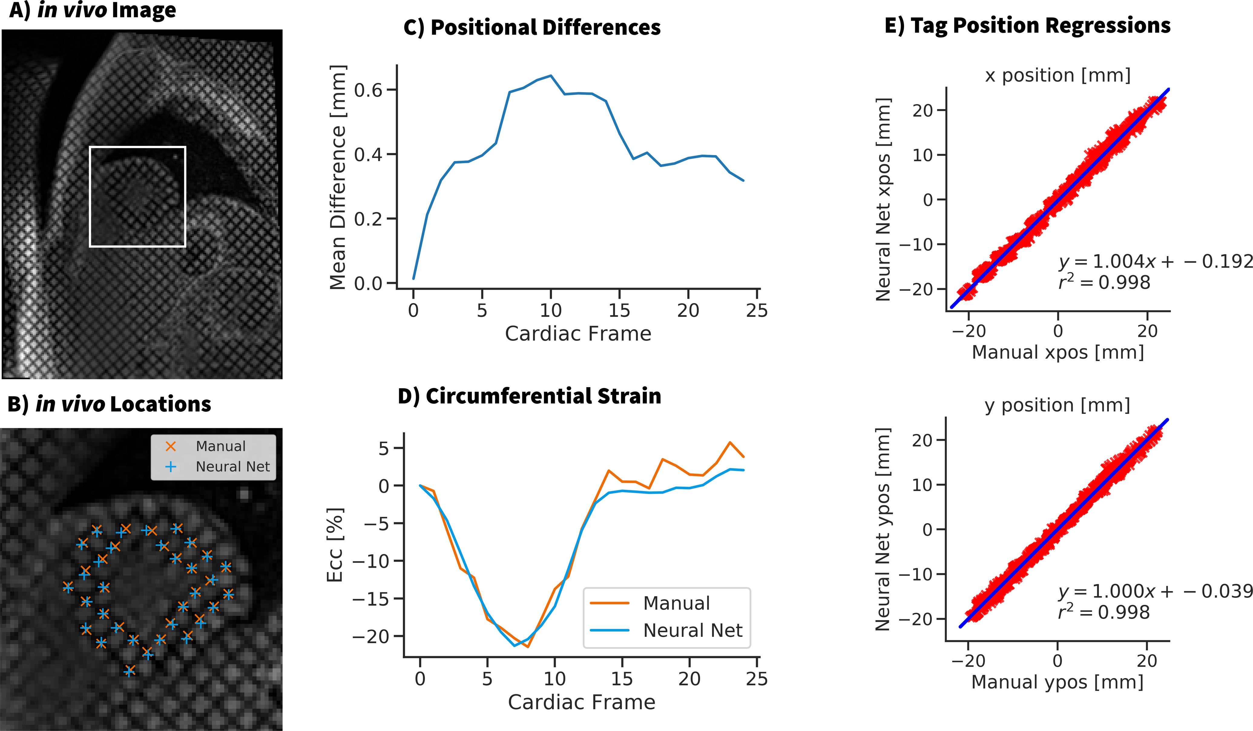
Tagging data from healthy pediatric volunteers (N=5, median age = 15Y, IRB approved, informed consent) was analyzed with the trained CNN. Ecc values were calculated from the detected tag locations. Tag motion paths and strains computed using the CNN were compared to the ones from manually tracked tag locations.
Results
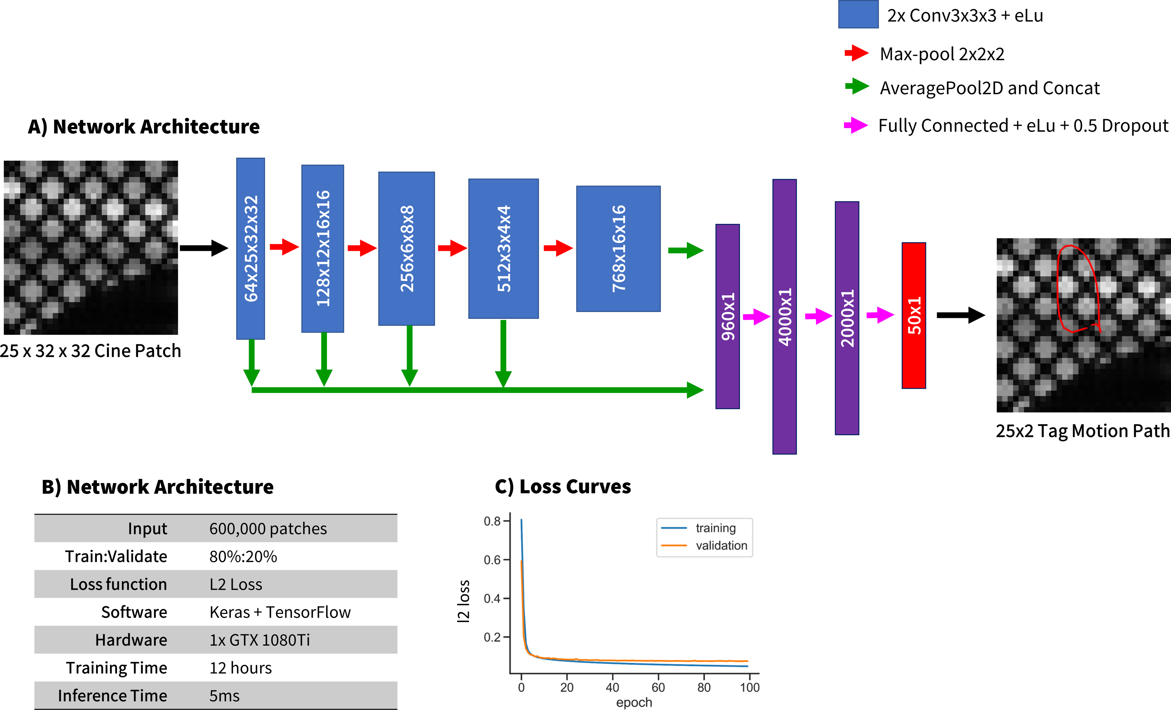
Details of the training process are shown in Fig 2 wherein 600,000 unique synthetic tag patches were generated and used for training. Fig 3 shows example images from the computational deforming cardiac phantom, as well as an overlay of our CNN calculated tag locations. RMSE of the tag locations was <0.4mm for SNR >10, and strain differences were <0.02. Very good agreement was seen in vivo between the CNN tagging and manual tag tracking (Fig 4). Tag locations were <1.0mm apart and strain values of the cardiac cycle agreed to within 0.02 Ecc.Discussion
Herein, a CNN was used to very quickly (<1s) and reliably track tag motion paths for the calculation of strains. The CNN was entirely trained using natural images with simulated motion paths and Bloch simulated tagging. By creating large amounts of training data with known displacement paths, the network can easily be retrained without the need to acquire large amounts of new training data and postprocess it. A computational deforming cardiac phantom with known strains was used to validate that the method works well for standard clinical SNR levels and resolutions. In vivo results showed very good agreement in tag motion paths, as well as calculated strains, compared to locations measured manually by an expert. Future work will incorporate the cardiac phantom into the training process, test the effect of adding real data into the training, combine segmentation into the network, and demonstrate use on a larger cohort with pathologies.Acknowledgements
NIH/NHLBI K25-HL135408 to LP
NIH R01 HL131823 to DBE
NIH R01 HL131975 to DBE
References
1. Young, A. A., Kraitchman, D. L., Dougherty, L. & Axel, L. Tracking and Finite Element Analysis of Stripe Deformation in Magnetic Resonance Tagging. IEEE Trans. Med. Imaging 14, 413–421 (1995).
2. Prince, J. L. & McVeigh, E. R. Motion Estimation from Tagged MR Image Sequences. IEEE Trans. Med. Imaging 11, 238–249 (1992).
3. Götte MJW, Germans T, Rüssel IK et al Myocardial strain and torsion quantified by cardiovascular magnetic resonance tissue tagging. Studies in normal and impaired left ventricular function. J Am Coll Cardiol (2006)
4. Osman NF, Kerwin WS, Mcveigh ER, Prince JL Cardiac motion tracking using CINE harmonic phase (HARP) magnetic resonance imaging. Magn Reson Med 42(6):1048–1060 (1999)
5. Ronneberger, O., Fischer, P. & Brox, T. U-net: Convolutional networks for biomedical image segmentation. in Lecture Notes in Computer Science (including subseries Lecture Notes in Artificial Intelligence and Lecture Notes in Bioinformatics) 9351, 234–241 (Springer Verlag, 2015).
6. Nam, H. & Han, B. Learning Multi-domain Convolutional Neural Networks for Visual Tracking. in Proceedings of the IEEE Computer Society Conference on Computer Vision and Pattern Recognition 2016-Decem, 4293–4302 (2016).
7. Verzhbinsky, I. A. et al. Estimating Aggregate Cardiomyocyte Strain Using In Vivo Diffusion and Displacement Encoded MRI. IEEE Trans. Med. Imaging (2019).
Figures