0684
Local Perturbation Responses: A tool for understanding the characteristics of advanced nonlinear MR reconstruction algorithms1Electrical and Computer Engineering, University of Southern California, Los Angeles, CA, United States
Synopsis
As MR image reconstruction algorithms become increasingly nonlinear, data-driven, and difficult to understand intuitively, it becomes more important that tools are available to assess the confidence that users should have about image reconstruction results. In this work, we suggest that a quantity known as the “local perturbation response” (LPR) provides useful information that can be used for this purpose. The LPR is analogous to a conventional point-spread function, but is well-suited to general image reconstruction methods that may have nonlinear and/or shift-varying characteristics. We illustrate the LPR in the context of several common image reconstruction techniques.
Introduction
Most classical MRI reconstruction methods possess both linearity and shift-invariant reconstruction characteristics. This simplicity means that it is easy for users to understand the confidence they should have in a reconstructed image, e.g., using concepts like point-spread functions to understand the expected spatial resolution characteristics1. This situation has changed in recent years, as MRI image reconstruction methods have become increasingly nonlinear and there is a trend towards “black-box” methods whose inner-workings and underlying assumptions can be difficult to understand. This means that there is a need for new tools that will allow users to easily evaluate the confidence they should have in an image that was reconstructed using a complicated nonlinear method.In this work, we suggest to use the local perturbation response (LPR), originally proposed to characterize spatial resolution in regularized tomography2,3, to understand the reconstruction characteristics of arbitrary MRI reconstruction methods. The LPR is analogous to a classical point-spread function, except that there is no expectation that the reconstruction behaves linearly.
Theory
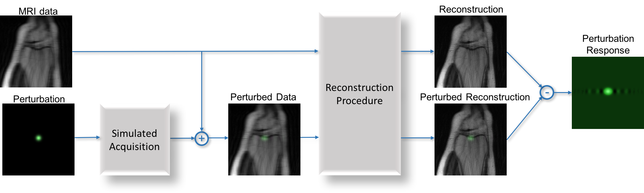
We assume that $$$\mathbf{x}$$$ is some original image of interest that we observe through some encoding operator $$$\mathbf{E}$$$, providing data $$\mathbf{d}=\mathbf{E}\mathbf{x}+\mathbf{n},$$ where $$$\mathbf{n}$$$ represents noise. We further assume that $$$\mathbf{x}$$$ is reconstructed from $$$\mathbf{d}$$$ using an arbitrary reconstruction method $$$f(\cdot)$$$, yielding an estimated image $$\hat{\mathbf{x}}=f(\mathbf{d}).$$ Ideally, we would assess the quality of $$$\hat{\mathbf{x}}$$$ by directly comparing it against the true image $$$\mathbf{x}$$$. However, this approach is generally impractical in real applications, since spending the time to acquire a fully-sampled reference image would defeat the purpose of developing the advanced image reconstruction method.Instead, the LPR attempts to assess image quality by applying a small perturbation to the image, and then observing how well that small perturbation is reconstructed by the image reconstruction method. Mathematically, if $$$\delta\mathbf{x}$$$ represents the small perturbation to the image in the image domain, the LPR is calculated by generating perturbed k-space data $$$\tilde{\mathbf{d}} = \mathbf{d}+\mathbf{E}\delta\mathbf{x}$$$, reconstructing the perturbed data using $$$f(\cdot)$$$, and comparing the result against the reconstruction obtained without a perturbation: $$\mathrm{LPR}=f(\mathbf{d}+\mathbf{E}\delta\mathbf{x})-f(\mathbf{d}).$$ This procedure is illustrated in Fig. 1. Importantly, this procedure can be implemented for arbitrary undersampled datasets, and does not require knowledge of any fully-sampled datasets. Ideally, if the reconstruction algorithm does a good job, the LPR will be a faithful reconstruction of the original perturbation. On the other hand, a substantial discrepancy between the LPR and the original perturbation would be a reason to doubt the results produced by the reconstruction method.
Methods
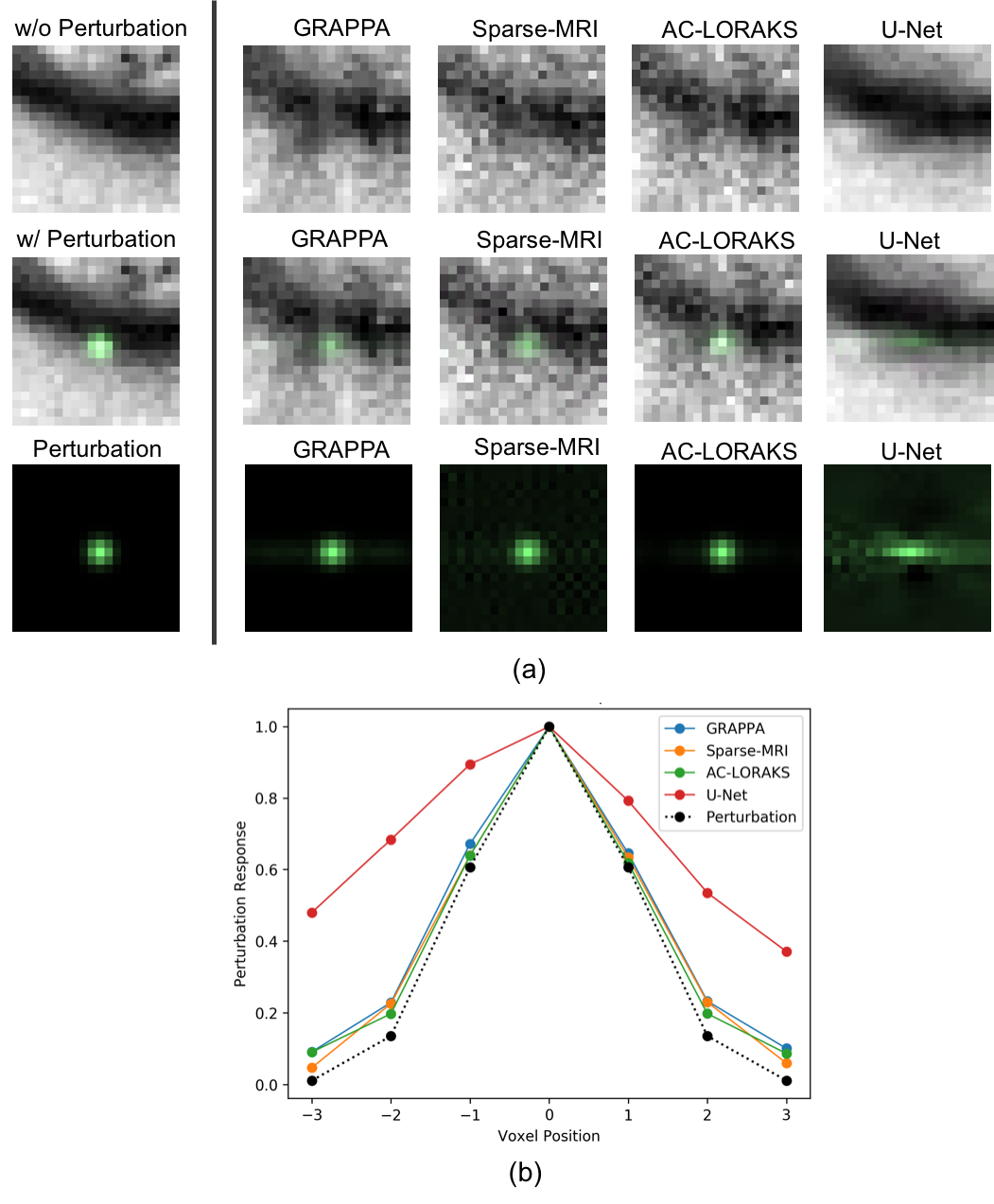
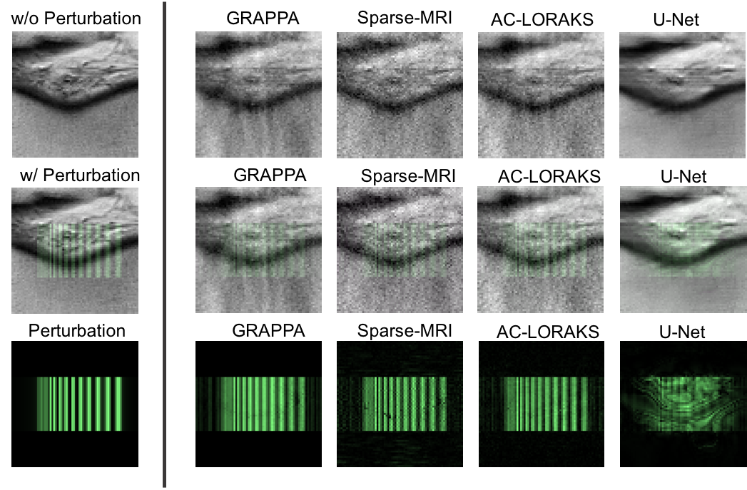
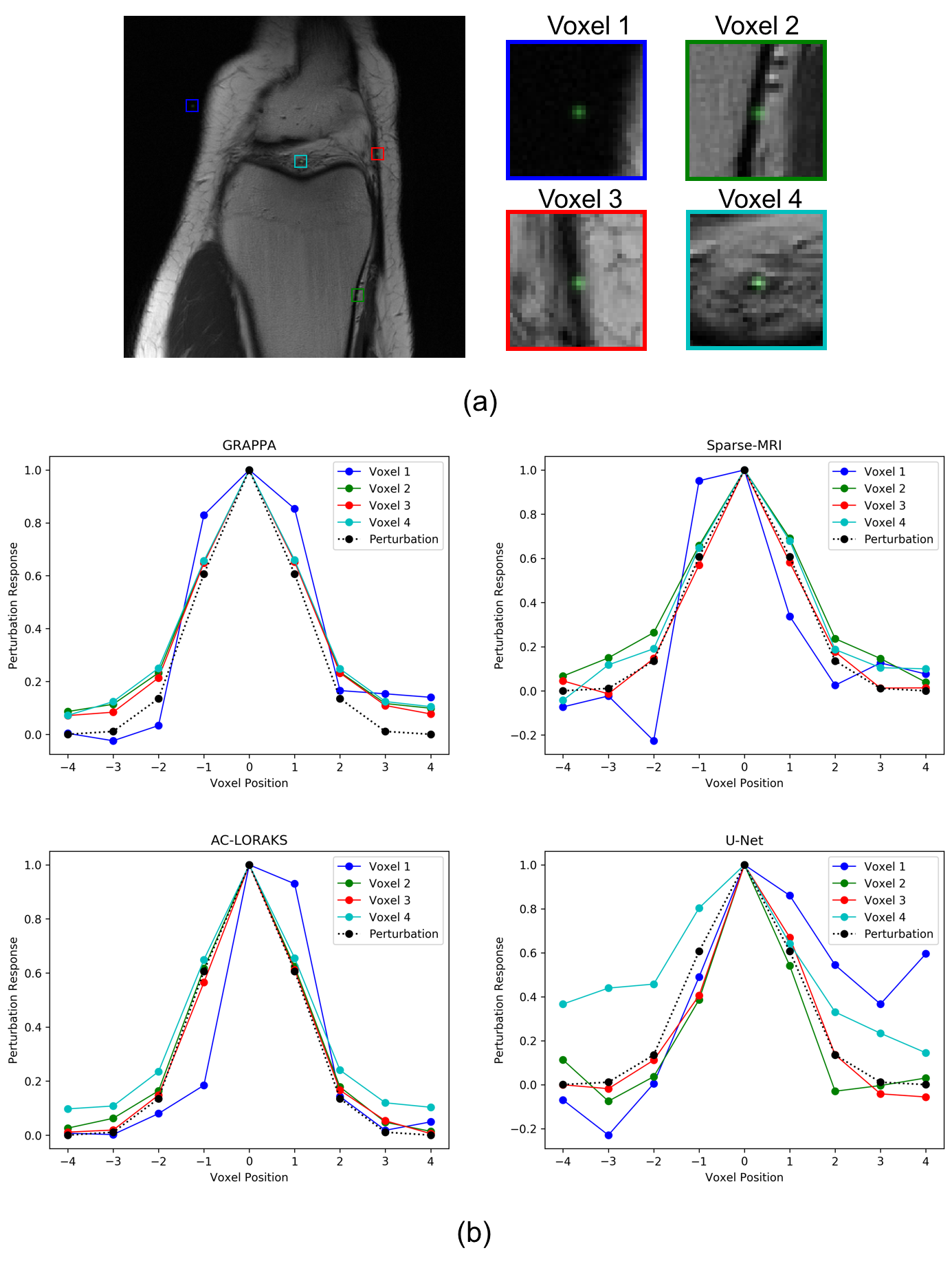
To assess the potential insights provided by LPRs, we computed LPRs for four different MRI reconstruction algorithms applied to one 15-channel dataset from the FastMRI database4, where the dataset was retrospectively undersampled to achieve an acceleration factor of 6. The reconstruction algorithms we considered included: GRAPPA5, Sparse-MRI6 using a SENSE-based forward model and total-variation regularization, AC-LORAKS7, and a deep-learning U-Net reconstruction architecture provided with the FastMRI data. The U-Net was trained using the FastMRI training dataset, comprising 19,878 fully-sampled MRI knee images. We considered two different kinds of perturbations (i.e., a small Gaussian blob as well as a striped resolution test-pattern). To test for shift-variance, we generated LPRs after shifting these perturbations to different spatial positions.Results
Results obtained with Gaussian blob perturbations are shown in Fig. 2, while results from the striped resolution test-pattern are shown in Fig. 3. The results demonstrate that these different reconstruction methods have different characteristics and capabilities when trying to reconstruct these perturbations. For these specific cases, the U-Net reconstruction method gives very poor reconstructions of the perturbation, suggesting that it may not be prudent to have too much confidence in those results. On the other hand, the other three methods all have reasonably good reconstructions of the perturbations, although each have their own unique characteristics. For example, the GRAPPA LPRs are generally a bit blurrier than the LPRs for Sparse-MRI and AC-LORAKS, suggesting potentially worse spatial resolution characteristics. AC-LORAKS also has an LPR that is slightly blurrier than the original perturbation. On the other hand, the Sparse-MRI LPRs appear to have some oscillatory features and other high-resolution features that may suggest a nonlinear interaction between the perturbation and the original data.Fig. 4 shows the results of computing LPRs of the same perturbation at different spatial locations. We can observe from this result that the LPRs are spatially-varying for all four methods, although spatial variation is most extreme for the U-Net and Sparse-MRI methods, while GRAPPA and AC-LORAKS have the least amount of spatial variation.
Discussion and Conclusions
We showed that the LPR can be used to provide insightful characterizations of advanced and potential nonlinear MR image reconstruction methods. Conceptually, the proposed LPR approach has similarities to stability tests proposed in recent work on deep learning MRI reconstruction8, although we approach perturbation analysis from a longstanding classical imaging perspective1,2. This classical approach is convenient because it can be used with arbitrary reconstruction methods (not just deep learning approaches), it is easy to interpret for users who are familiar with the concept of a point-spread function, and it can be applied to arbitrary undersampled datasets (i.e., fully-sampled reference data is not required).Acknowledgements
This work was supported in part by research grants NSF CCF-1350563, NIH R01 MH116173, NIH R01 NS074980, and NIH R01 NS089212, as well as a USC Viterbi/Graduate School Fellowship.References
[1] Liang ZP, Lauterbur PC. Principles of magnetic resonance imaging: a signal processing perspective. IEEE Press, 2000.
[2] Fessler JA, Rogers WL. “Spatial resolution properties of penalized-likelihood image reconstruction: space-invariant tomographs.” IEEE Trans. Image Process., 5(9), 1346-1358, 1996.
[3] Ahn S, Leahy RM. “Analysis of resolution and noise properties of nonquadratically regularized image reconstruction methods for PET.” IEEE Trans. Med. Imag., 27(3), 413-424, 2008.
[4] Zbontar J, Knoll F, Sriram A, Muckley MJ, Bruno M, Defazio A, Parente M, Geras KJ, Katsnelson J, Chandarana H, Zhang Z, Drozdzal M, Romero A, Rabbat M, Vincent P, Pinkerton J, Wang D, Yakubova N, Owens E, Zitnick CL, Recht MP, Sodickson DK, Lui YW. “fastMRI: An open dataset and benchmarks for accelerated MRI.” arXiv:1811.08839, 2018.
[5] Griswold MA, Jakob PM, Heidemann RM, Nittka M, Jellus V, Wang J, Kiefer B, Haase A. “Generalized autocalibrating partially parallel acquisitions (GRAPPA).” Magn. Reson. Med., 47(6), 1202-1210, 2002.
[6] Lustig M, Donoho D, Pauly JM. “Sparse MRI: The application of compressed sensing for rapid MR imaging.” Magn. Reson. Med., 58(6), 1182-1195, 2007.
[7] Haldar JP. “Autocalibrated LORAKS for fast constrained MRI reconstruction.” in Proc. IEEE ISBI, 2015, pp. 910-913.
[8] Antun V, Renna F, Poon C, Adcock B, Hansen AC. “On instabilities of deep learning in image reconstruction - Does AI come at a cost?” arXiv:1902.05300, 2019.
Figures