Purpose:

Echo Planar Imaging (EPI) and balanced Stead-Stated Free Precession (bSSFP) are frequently used pulse sequences in functional magnetic resonance imaging (fMRI). The capability to acquiring the brain volume within seconds makes them a significant, non-invasive tool for probing dynamic changes in the blood-oxygenation-level-dependent (BOLD) response. Both sequences are sensitive to magnetic field (B₀) inhomogeneity. Perturbations in the field result in signal loss, banding artifact, and geometric distortion.

Therefore, correcting geometric distortions in functional images increases the accuracy of co-registration to structural MR. Correcting distortion using acquired Field maps has been shown to improve registration¹. Subject movement can change the pattern of B₀ inhomogeneity. However, it’s impractical to acquire a field map matches every possible movement during functional data acquisitions. Previously, field probes have been used to estimate the dynamic of field fluctuation and correct for this, but they cannot fully estimate B₀ inside the brain since they are placed outside the brain.²

Here, we estimate the motion-related B₀ variations using a Fourier-based dipole-approximation method^3-5. A 4-class susceptibility model (air, bone, fat, and water) is calculated using a combined ultrashort-echo-time/Dixon (UTE/Dixon) MRI sequence.

Method:

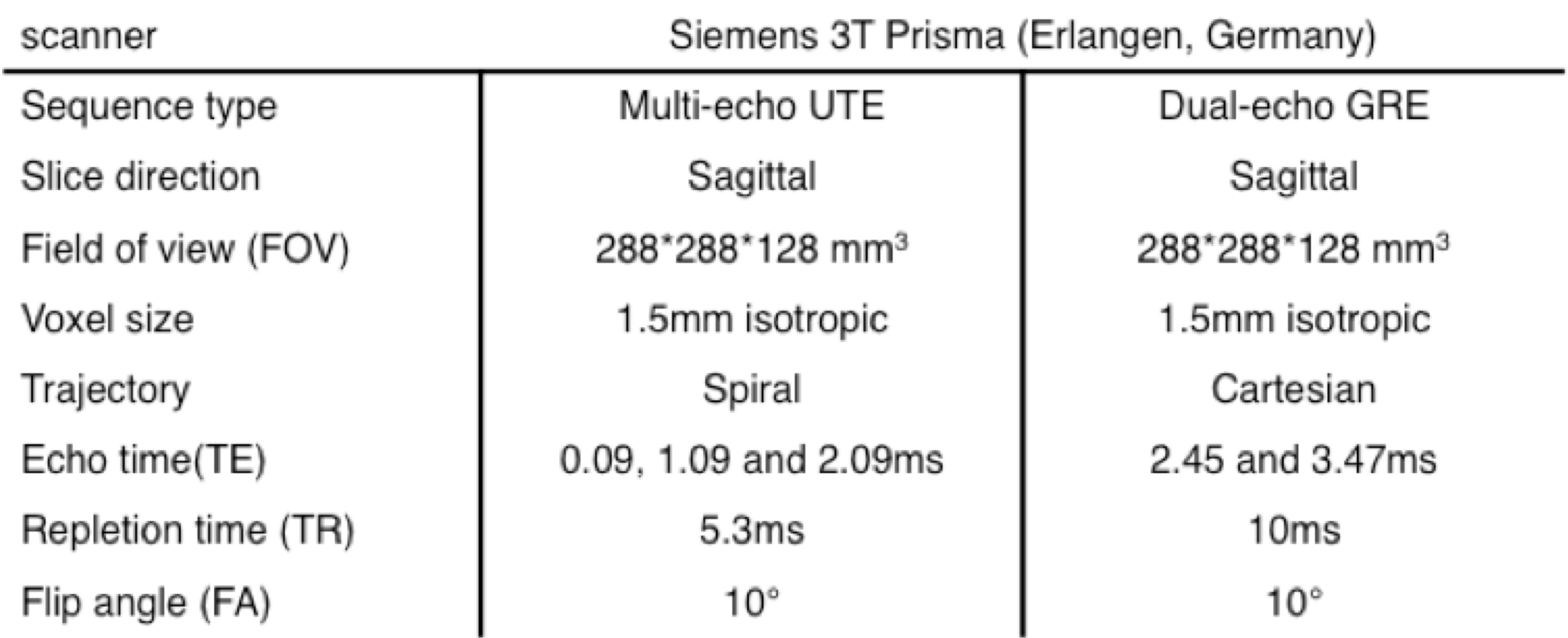
A 3D UTE sequence with spiral trajectory was used after shimming the entire volume with the scanner’s second-order spherical harmonic (SH) shim. A dual-echo GRE sequence was used to measure reference B₀ maps and scanner’s background inhomogeneity. The detailed MR sequence parameters are listed in Table 1.

A 4-classes (air, bone, fat, and water) susceptibility model was implemented in MATLAB (MathWorks) (Flow chart, Figure2). The air mask, including cavities, was created using an empirically determined magnitude threshold6 of the first and third echo as well as by morphologic filtering. The cortical bone was segmented using inverse of the transverse effective relaxation rate (R2*) estimated from all three echoes, where the cortical bone has high R2* values (R2*bone≥0.3ms^-1)⁷. The bone structures were segmented using an empirically determined threshold and cleaned up using morphologic filtering. The remaining tissue was assigned a relative water-fat fraction, determined through a two-point Dixon decomposition⁸ using the second (out-phase) and third echo (in-phase). The water-fat fraction r is a normalized map⁹, ranging from -1(purely fat) to +1 (purely water). Finally, the susceptibility map of mix water and fat voxel was then calculated from the relative water-fat fraction r using the linear mapping as follow:$$\chi_{water-fat map} = \frac{(1+r)}{2}\times\chi_{water-mean}+\frac{(1-r)}{2}\times\chi_{fat-mean}$$ Then, the binary air and bone mask were applied to have the subject-specific susceptibility model $$$(\chi_{water-mean}\approx-9.2ppm, \chi_{fat-mean}\approx-10ppm, \chi_{bone}\approx-11.3ppm, \chi_{air}\approx3.6ppm)$$$. A Fourier-based method was then used to calculate the estimated field map from subject-specific susceptibility model for position 1.

Two different head positions were measured to demonstrate field map predicting for motion-induced B₀ variations. The measurement was repeated with the head in a second position without further shimming. For the second position, two alternative strategies were used for predicting the field maps. 1) From the measured position 1 field map using the position calculated transformation matrix (FSL¹⁰ FLIRT¹¹ toolbox, a 12-degree affine transformation) and tri-linear interpolation. 2) From the susceptibility model using the transformation matrix followed by a forward calculation of the expected field map.

Result:

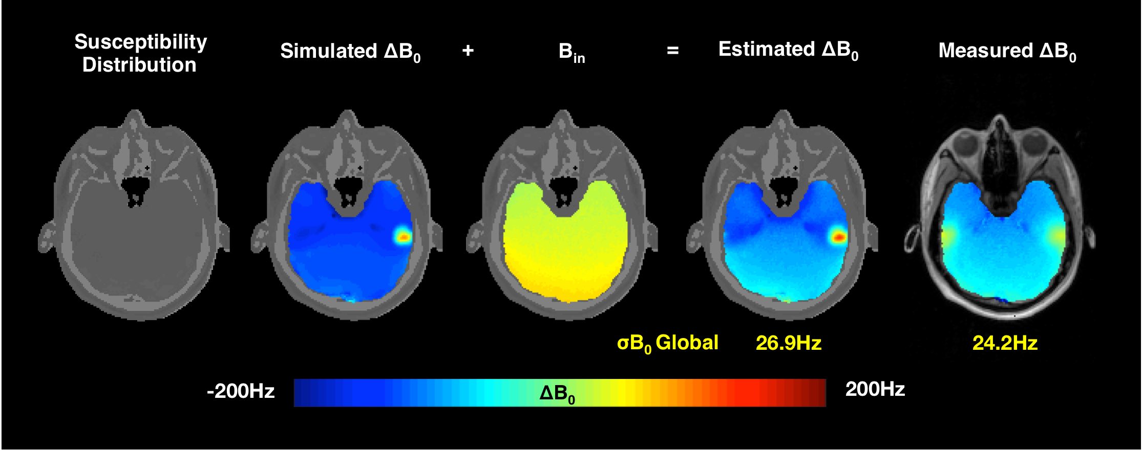
Figure 3 shows the field maps estimated from the UTE susceptibility model for the first position. Estimated field map has a similar deviation of inhomogeneity (σB₀ = 26.9Hz) in comparison to the measured one (σB₀ = 24.2 Hz). Figure 4 shows the discrepancy between the estimated field map and the measured field map for motion-induced B₀ variations. The field map difference for strategy 1 was calculated between the measured position 2 field map and a field map co-registered from position 1. The difference of the forward strategy 2 was calculated between the estimated field maps. The σB₀ of the field map difference using the proposed method is 2.7Hz, compared to 10.6Hz of the measured field map.

Discussion:

In this study, we further improved the UTE method to estimate the field map¹², with 4-class tissue segmentation. The σB₀ of estimated and measured field map are in good agreement. The forward prediction strategy has a smoother difference field map, compared with the measured strategy. The potential reasons would be 1) B₀-variation induced by the respiration cycle was not taken into consideration for forwarding strategy; 2) The tri-linear interpolation of the position 1 field map would smooth the field map. In the future, the subject motion time series could be captured using a motion camera. However, the motion camera only recorded the rigid body motion from the skull. The relative motion between the skull and neck needs to be further investigated.

Acknowledgements

This work was supported by DFG SCHE658/13 and the Max Planck Society.