Introduction

Fast and accurate $$$B_1^+$$$-mapping is a very important prerequisite at high and ultrahigh field (UHF) for various applications including the correction for varying flip angle distribution in qMRI^1,2 and pTx^3,4. A very promising approach to directly measure the magnitude of the $$$B_1^+$$$-field is the method of Bloch Siegert (BS)⁵. However, at UHF 3D BS $$$B_1^+$$$-mapping is in particular limited by high energy deposition of multiple off-resonant RF-pulses resulting in unacceptable long acquisition times. To overcome these problems we recently proposed a reconstruction algorithm for highly under-sampled BS data based on variational modelling⁶, which was evaluated on 3T. The much more pronounced spatial RF-field variations and energy deposition at 7T makes an investigation according the performance and accuracy of the reconstruction algorithm necessary. In this work, the performance of the proposed BS mapping technique is investigated for phantom and in-vivo at 7T.

Theory and Medhods

The variational reconstruction algorithm consists of a two-step procedure, defined by solving two optimization problems. In the first step a TGV-regularization term^7,8, which enforces piecewise smooth solutions, is applied to reconstruct the magnitude and phase of the underlying image. In the second step a smoothness constraint is applied to enforce the spatial smoothness of the underlying $$$B_1^+$$$-field defined as follows:
$$\hat{u}=\arg\min_u\frac{\lambda}{2}\parallel\,k_+-\mathcal{F}\left(u\right)\,\parallel_2^2+TGV\left(u\right)$$
$$\hat{v}=\arg\min_v\frac{\mu}{2}\parallel\,k_--\mathcal{F}\left(\hat{u}\,\cdot\,v\right)\,\parallel_2^2+\parallel\nabla\,v\parallel_2^2=e^{-j2\phi_{BS}}$$
For further details we refer to⁶.

A spherical phantom and a healthy subject were scanned on a 7T system (Magnetom, Siemens, Erlangen, Germany) with a 1Tx32Rx head coil (Nova Medical, Wilmington, USA) according to the local IRB approved protocol. The following scan parameters were used to acquire the phantom data: FOV=200x200mm, slab thickness=150mm, acquisition matrix=128x128x30, $$$TR/TE=160/15ms$$$, $$$T_{pulse}=10ms$$$, $$$\alpha_{BS}=1000°$$$,$$$f_{BS}=5kHz$$$. The in-vivo dataset was acquired using: FOV=256x192mm, slab thickness=80mm, acquisition matrix=128x96x16, $$$TR/TE=377/10ms$$$ and 25% slice oversampling. A Fermi shaped BS pulse with duration $$$T_{pulse}=7ms$$$, $$$\alpha_{BS}=600°$$$ on-resonant equivalent flip angle and a resonance offset of $$$f_{BS}=4kHz$$$ leading to a pulse constant $$$K_{BS}=70.93rad/G^2$$$ was used. The regularization parameters $$$\mu$$$ and $$$\lambda$$$ were adjusted doing a parameter sweep to $$$\mu=1.1\cdot 10^{-2}$$$ and $$$\lambda=10$$$.
Data were retrospectively subsampled using a block pattern with different sizes, where only $$$n\times m$$$ lines in k-space center were acquired as described in⁶. The reconstruction results were compared to a fully sampled reference and for each result the difference map was computed. Each result was further evaluated by mean absolute error (MAE), median value (medAE) and 90% quantile over a region of interest inside the subject’s brain.

Results and Discussion

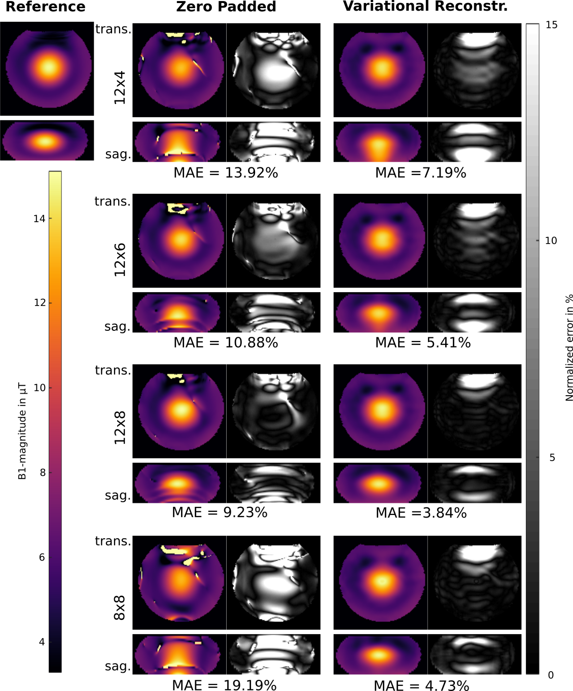
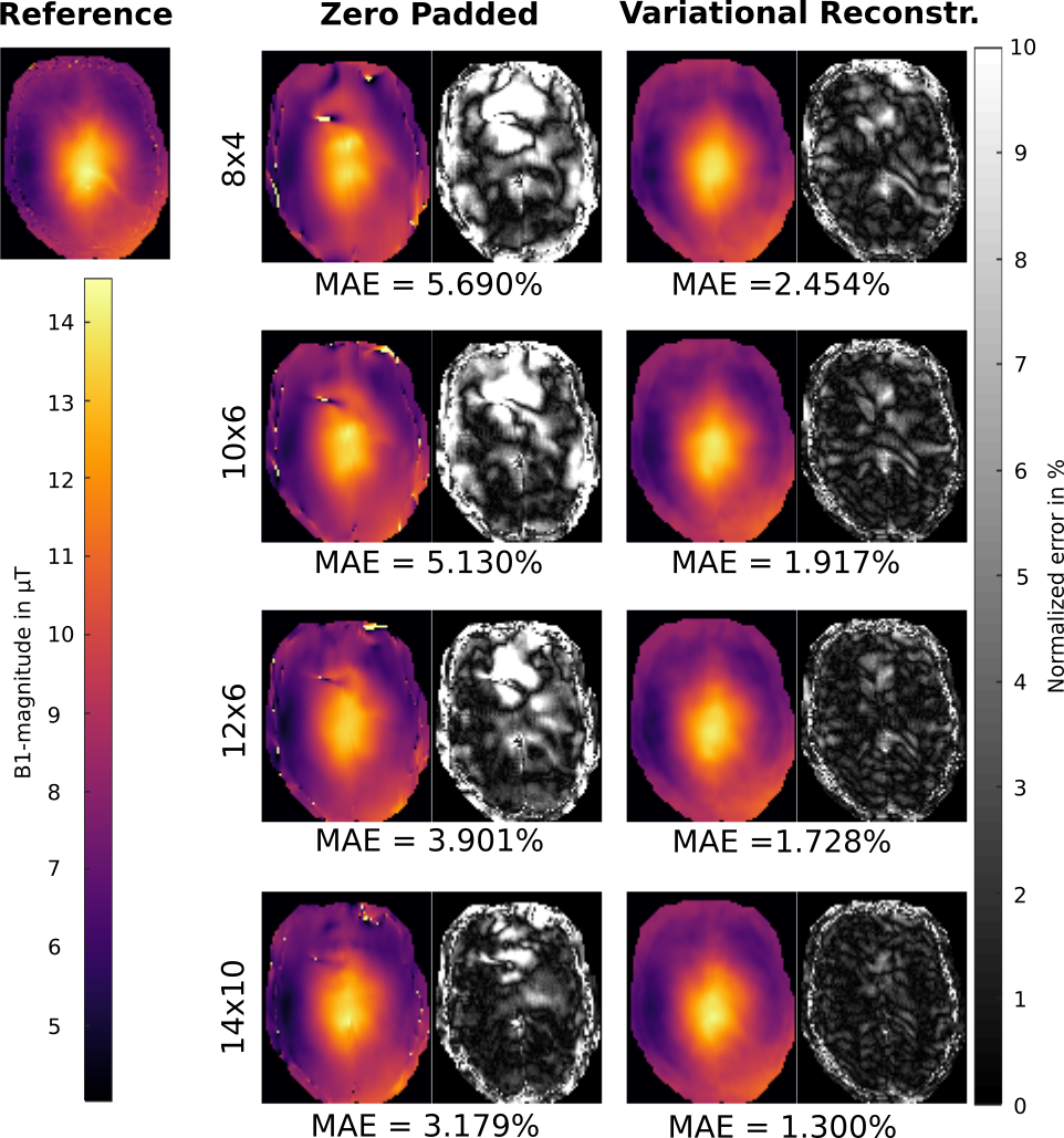
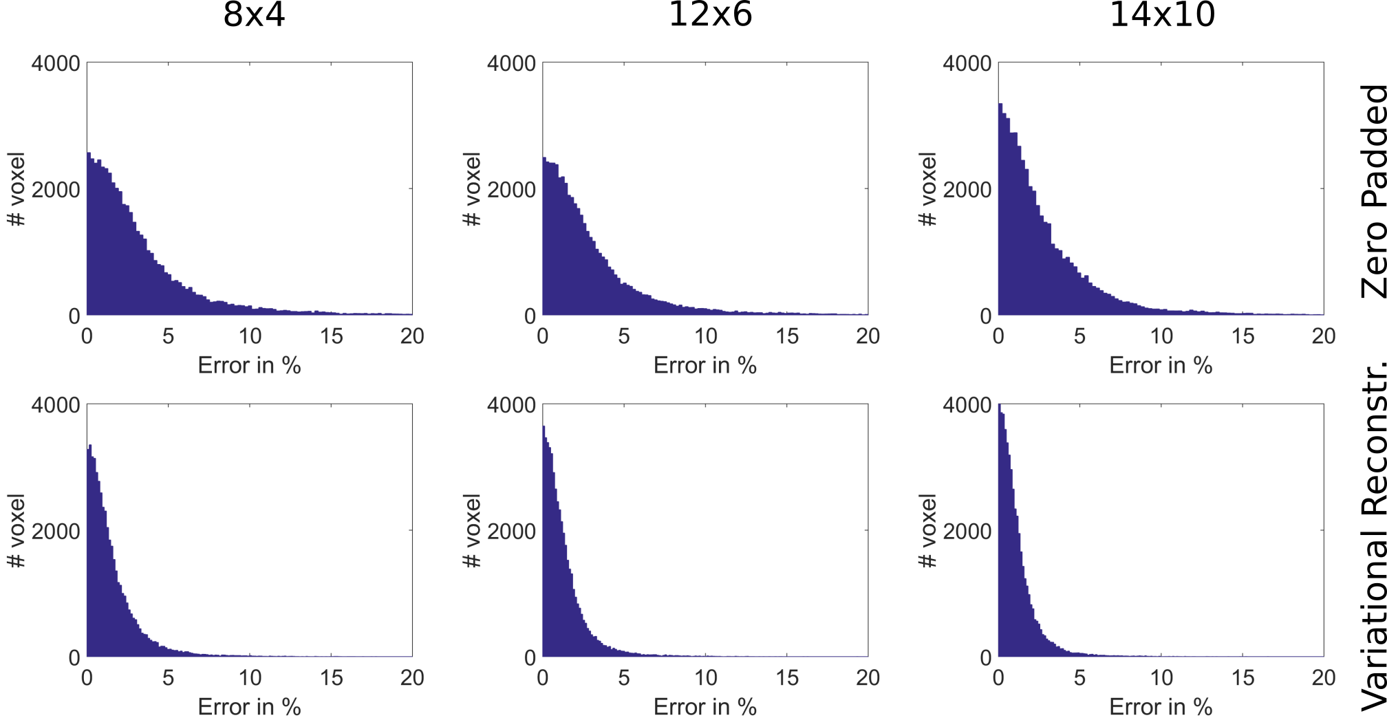
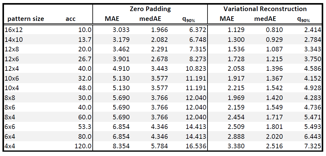
Figure 1 (phantom) and 2 (in-vivo) show the reconstructed 3D $$$B_1^+$$$-maps after zero filling and the proposed TGV approach for 4 different pattern sizes together with a fully sampled reference. The difference map and the MAD indicate low errors in both cases for the proposed TGV reconstruction. The limitation of the TGV method can be seen in the sagittal plane of Figure 1 ($$$12\times 4$$$ pattern) where the $$$B_1$$$-hotspot in the center of the phantom is blurred out in z-direction as a result of insufficient k-space data, although zero filling resulted in much more severe artifacts. For in-vivo measurements such a blurring was not observed. It is remarkable that using only 1.7% of the k-space (pattern size of $$$8\times 8$$$) the average error stays below 5%. Table 1 lists the MAE, medAE and the 90% quantile for a range of under-sampling pattern sizes and the resulting acceleration factor $$$acc$$$ for the in-vivo measurements. With the pattern size of 10x6 (about 2% of the fully-sampled data) we can reach an average error below 2% over the whole FOV in a scan time of about 45s with the given TR at 7T. Figure 3 shows the error histograms over the whole brain region inside the cortical bone structure for three pattern sizes for zero padding and the variational reconstruction results. The narrowing in the histograms for the results gained with the variational reconstruction clearly demonstrates the increased accuracy. Compared to the results at 3T reported in⁶, the mean error increased for all pattern sizes from below 1% at 3T to about 2% for medium pattern sizes. For smaller pattern sizes the error increases drastically, indicating that the more pronounced field variations at 7T cannot be resolved any more. This is further supported by an increase of the optimal regularization parameter $$$\mu$$$ by more than an order of magnitude from $$$5\cdot 10^{-4}$$$ to $$$1.1\cdot 10^{-2}$$$, indicating that more data weighting is necessary to resolve the field variations.⁶ Even though the RF energy deposition increases heavily, a minimum acquisition time in the order of 45s-1min is possible.

Conclusion

In this study we successfully applied the proposed algorithm on 7T phantom and in-vivo data. The mean error was reduced for both in-vivo and phantom measurements compared to zero padding which allows the acquisition of accuate 3D $$$B_1^+$$$-maps in about 45s.

Acknowledgements

The authors gratefully acknowledge support from NVIDIA Corporationfor providing GPU computing hardware.