INTRODUCTION

Spiral or UTE sequences are susceptible to variations in dynamic gradient response caused by eddy currents, timing inaccuracies, or gradient amplifier non-linearities that cause a mismatch between expected and actual k-space trajectory. Linear effects, such as caused by eddy currents, can be taken into account by correcting the gradient waveform using a measured or modeled gradient impulse response function (GIRF) for calculation of accurate trajectories [1,2]. Non-linear effects can be introduced by the gradient amplifiers, whose actively controlled feedback loops have limited temporal resolution and may cause slight deviations from a linear response. The resulting errors are reproducible but differ for every gradient waveform and are thus hard to predict. As a mitigation, additional hardware can be employed to directly measure gradient fields during imaging, e.g. with a hardware field camera [3] or using inductive methods [4]. To avoid the need for additional hardware, we propose to measure the gradient amplifier output currents concurrently with imaging. Convolving the currents with the measured current-to-gradient impulse response function (CGIRF) leads to improved accuracy of the trajectory calculation. We demonstrate the CGIRF method in 2D spiral imaging and compare with results obtained from a model-based as well as a conventional GIRF approach.

METHODS

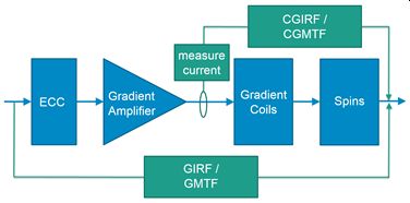
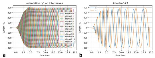
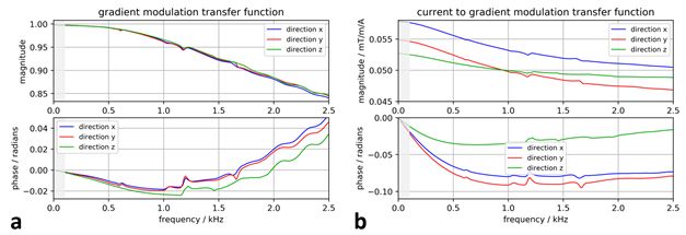
Figure 1 compares the conventional GIRF approach with the suggested CGIRF method. Conventionally, the gradient modulation transfer function (GMTF) of the complete gradient chain is modeled or measured, and the field response to an input waveform is calculated using this transfer function. The CGIRF method now measures the true amplifier output current during imaging. With knowledge of the transfer function between output currents and fields (CGMTF), which mainly represents the behavior of the gradient coil, a k-space trajectory can be calculated that contains the full dynamics of the applied currents that generate the gradient fields. A spiral scan of a single transverse slice (xy plane) was performed on a clinical 3 T system (Ingenia, Philips, The Netherlands). The FoV was 230x230 mm², slice thickness was 8 mm, and the in-plane scan resolution was 1 mm. Reconstruction was performed on a grid of 320x320 pixels. TE was 2 ms, TR was 500 ms, and the flip angle was 20°. The spiral trajectory had 12 interleaves, each with an acquisition window of 18.7 ms. The scan was repeated twice to sequentially record the amplifier output currents (Ix, Iy) shown in Figure 2. Current measurements were started shortly before gradient ramp up to be able to determine shim currents that need to be removed before further processing. Reconstructed images have been corrected for B0 inhomogeneity based on ΔB0 maps that were acquired prior to the imaging experiment. For later GMTF correction, the gradient waveforms sent to the gradient chain as well as the gradient amplifier output currents were exported to disk. The 3D transfer functions for all three gradient channels were measured using a 3D thin-slice method5 on a spherical phantom (Ø 24 cm) filled with aqueous CuSO4 solution. The method selects 4 slices in each direction, which were sub-partitioned into 5x5 voxels using phase-encoding. A through-slice chirp test gradient with a bandwidth of 30 kHz and a duration of 80 ms was applied in each direction, creating sets of 100 voxels which enabled the extraction of the spatial harmonic components of the gradient response [2]. Here, only the direct gradient terms were used for calculation of the GMTF (division of the response spectrum by the spectrum of the test waveform) and the CGMTF (division of the response spectrum by the spectrum of the measured gradient amplifier output currents) shown in Figure 3. By applying an inverse real FFT on the transfer functions, the time domain GIRFs and CGIRFs were obtained. For correction of all spiral interleave trajectories, the gradient waveforms sent to the gradient chain were convolved with the respective direct 1st order response functions for the Gx and Gy channel. The k-space trajectories were then obtained by integration and were passed to the spiral gridding routine in reconstruction, followed by ΔB0 de-blurring.

RESULTS AND DISCUSSION

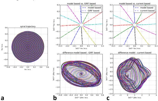
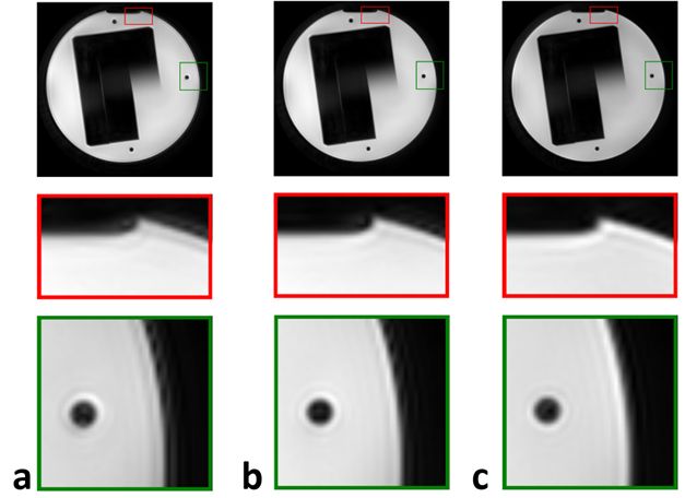
Figure 4 compares the k-space trajectory obtained using GIRF and CGIRF correction with the standard trajectory that is calculated using a simple low-pass filter model for the gradient chain. The difference plots show that the linear GIRF corrections have ellipsoidal shape in k-space, while the non-linear CGIRF corrections correspond to more complicated higher order structures. Figure 5 shows the respective reconstructed images. Since all three approaches compensate for the effect of the gradient chain, differences between the methods are small, but visible. Both, the GIRF and CGIRF approach lead to better depiction of small structures. With respect to the signal level outside the phantom, the GIRF approach shows an improvement, but the CGIRF image delivers the best edge depiction.

CONCLUSION

Image reconstruction based on trajectories derived from measured currents corrected with the current-to-gradient impulse response function provide image quality improvements in spiral imaging due to the removal of amplifier non-linearities as well as linear eddy current effects. As a fully measurement-based approach, no assumptions on the gradient waveform and the gradient chain characteristics are required.

Acknowledgements

No acknowledgement found.