0619
PILOT: Physics-Informed Learned Optimal Trajectories for Accelerated MRI1CS, Technion, Haifa, Israel, 2Technion, Haifa, Israel, 3University of Waterloo, Waterloo, ON, Canada
Synopsis
We propose a novel approach to the learning of conjoint acquisition and reconstruction of MRI scans. The acquisition is encoded in the form of general k-space trajectories, which constrained to obey the hardware requirements (peak currents and maximum slew rates of magnetic gradients). We demonstrate the effectiveness of the proposed solution in both image reconstruction and image segmentation, reporting substantial improvements in terms of acceleration factors and the quality of these end tasks. To the best of our knowledge, our proposed algorithm is the first to do data- and task-driven learning over the space of all physically feasible k-space trajectories.
Introduction
Multiple studies have focused on the development of both physical (acquisition) and post-processing (reconstruction) approaches for accelerated acquisition of MRI scans (1;2;3;4). Recently, there is increasing attention towards addressing this problem as simultaneous optimization of acquisition and reconstruction schemes (5;6;7;8) exploiting the modern deep learning frameworks. However, these works were limited to the specific scenario of Cartesian sampling trajectories. In this work, we introduce PILOT, a novel approach to learn general k-space trajectories jointly with the reconstruction models. We explicitly constrain the trajectories to obey a set of predefined hardware constraints: peak current and maximum slew rates of the magnetic gradients. We demonstrate the proposed method is general and be simply adapted to different end-tasks with substantial improvements in the acceleration rate vs. performance trade-offs. We present results on two end-tasks, MRI image formation, and tumor segmentation at different acquisition times. To the best of our knowledge, ours is the first work to do end-to-end data- and task-driven learning over the space of all physically feasible MRI k-space trajectories. In this work, our major focus is on obtaining the optimal single-shot 2D trajectory for a given task; however, our method can be simply generalized also to a multi-shot setting and to 3D trajectories (13).Method
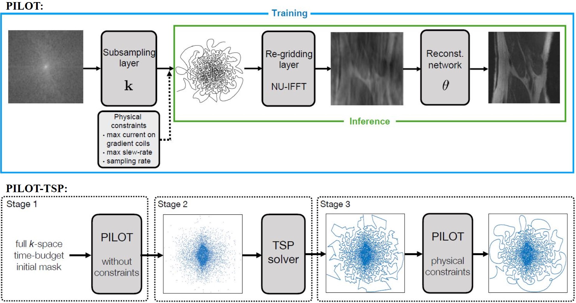
We view our approach as a single neural network combining the forward (k-space sub-sampling in our case) and the inverse (reconstruction) models (see Fig. 1). The input to the model is the fully sampled k-space. The input is faced by a sub-sampling layer modeling the data acquisition along a k-space trajectory (emulated by bi-linear interpolation), a regridding layer producing an image on a Cartesian grid in the space domain (NU-IFFT), and an end-task model operating in the space domain and producing a reconstructed image (reconstruction task) or a segmentation mask (segmentation task). The decimation rate is defined to be the ratio between the number of sub-sampled points and the number of points in the full k-space. The training of the proposed pipeline is performed by simultaneously learning the trajectory k and the parameters of the task model. The loss function is composed of two terms: a task-fitting term and penalties enforcing the physical constraints. The aim of the task-fitting term is to measure how well the specific end task is performed. For the reconstruction task, we define this term to be the L1 norm between the output of the task model and the ground-truth image, derived from the fully sampled k-space. For the segmentation task, we use the pixel-wise cross-entropy between the model-estimated segmentation map and the ground truth segmentation map. The second term in the loss function applies to the trajectory k only and penalizes for the violation of the physical constraints. We define the penalties as the hinge loss of the form max(0, |k|-vmax) and max(0,|k|-amax) summed over the trajectory coordinates, where vmax and amax are derived from the physical constraint of peak-current (Gmax) and maximum slew-rate (Smax) respectively. These penalties remain zero as long as the solution is feasible and grows linearly with the violation of each of the constraints.PILOT - TSP: When initialized with one of the standard single-shot trajectories (EPI, spiral, etc), PILOT maintains the general shape of its initialization with moderate, local modifications (see Fig. 4, left & middle columns). In order to alleviate this effect, we introduce PILOT-TSP, an extension of PILOT for optimizing trajectories from random initialization (TSP: Traveling Salesman Problem) (10). Translated to our terminology, TSP aims at finding an ordering of given k-space locations such that the path connecting them has minimal length. Since TSP is NP-hard, we used a greedy approximation algorithm (11) for solving it. In PILOT-TSP, we first optimize for the best-unconstrained solution and then find the closest solution satisfying the constraints using PILOT (see the scheme in Fig. 2).
Results and discussion
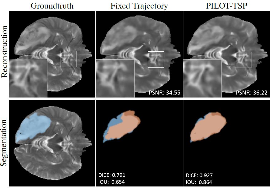
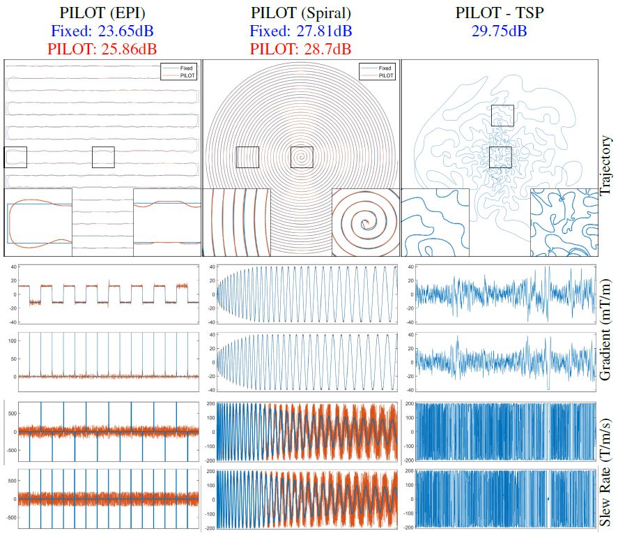
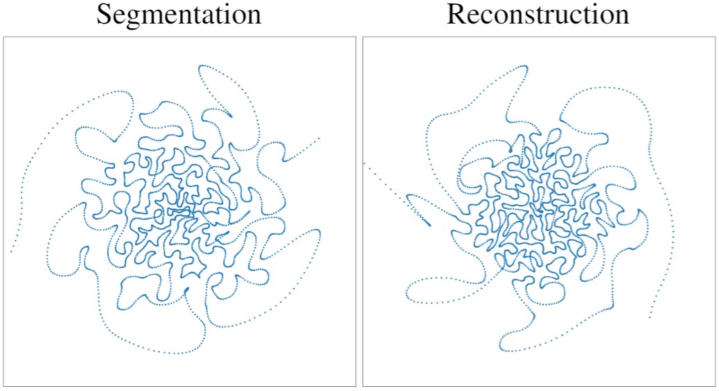
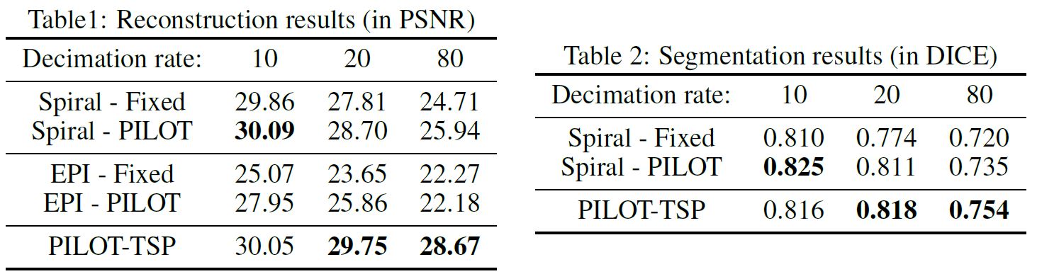
The following physical constraints were used in all our experiments: Gmax=40 mT/m for the peak gradient and Smax=200 T/m/s for the maximum slew-rate. We used two datasets in the preparation of this report: the NYU fastMRI knee-scans (3), and the brain tumor segmentation dataset from (12). We observed that starting from an infeasible trajectory (EPI), PILOT learns a feasible trajectory that, in most cases, outperforms the baseline infeasible trajectory, and sometimes preserves the performance at the level of the (infeasible) baseline while making the trajectory feasible under the chosen physical constraints (as evaluated quantitatively across decimation rates and presented in Table 1, second row). Starting from a feasible trajectory (spiral), PILOT learns, for both tasks and across decimation rates, a more optimal trajectory that is also physically feasible. The optimal trajectory demonstrates significant improvement over the fixed counterparts (Table 1, first row & Table 2). A visual comparison of the fixed and learned trajectories is given in Fig. 4. Finally, we show a superior performance of the arbitrarily initialized PILOT-TSP, across tasks and decimation rates (cf. Tables 1&2; bottom row in Fig. 3). It is particularly interesting to observe the variations in the trajectories learned for segmentation and reconstruction (Fig. 4). We can see that the reconstruction trajectory is more centered around the DC frequency, whereas the segmentation trajectory tries to cover higher frequencies.Acknowledgements
No acknowledgement found.References
1. K. Hammernik, T. Klatzer, E. Kobler, M. P. Recht, D. K. Sodickson, T. Pock, and F. Knoll, “Learning a variational network for reconstruction of accelerated mri data,” Magnetic resonance in medicine, vol. 79, no. 6, pp. 3055–3071, 2018.
2. J. Sun, H. Li, Z. Xuet al., “Deep admm-net for compressive sensing mri,” advances in neural information processing systems, 2016.
3. J. Zbontar, F. Knoll, A. Sriram, M. J. Muckley, M. Bruno, A. Defazio, M. Parente, K. J. Geras,J. Katsnelson, H. Chandaranaet al., “fastmri: An open dataset and benchmarks for accelerated MRI,”arXiv preprint arXiv:1811.08839, 2018.
4. C. Lazarus, P. Weiss, N. Chauffert, F. Mauconduit, L. El Gueddari, C. Destrieux, I. Zemmoura,A. Vignaud, and P. Ciuciu, “Sparkling: variable-density k-space filling curves for acceleratedt2*-weighted mri,” Magnetic Resonance in Medicine, vol. 81, no. 6, pp. 3643–3661, 2019.
5. S. Vedula, O. Senouf, G. Zurakhov, A. Bronstein, O. Michailovich, and M. Zibulevsky, “Learn-ing beamforming in ultrasound imaging,” in proceedings of The 2nd International Conference on Medical Imaging with Deep Learning, ser. Proceedings of Machine Learning Research, vol.102. PMLR, July 2019, pp. 493–511.
6. O. Menashe and A. Bronstein, “Real-time compressed imaging of scattering volumes,” in2014IEEE International Conference on Image Processing (ICIP). IEEE, 2014, pp. 1322–1326.
7. H. Haim, S. Elmalem, R. Giryes, A. M. Bronstein, and E. Marom, “Depth estimation from a single image using deep learned phase coded mask,” IEEE Transactions on ComputationalImaging, vol. 4, no. 3, pp. 298–310, 2018.
8. T. Weiss, S. Vedula, O. Senouf, A. Bronstein, O. Michailovich, and M. Zibulevsky, “LearningFast Magnetic Resonance Imaging,”arXiv e-prints, p. arXiv:1905.09324, May 2019.
9. T. Weiss, O. Senouf, S. Vedula, O. Michailovich, M. Zibulevsky, and A. Bronstein, “PI-LOT: Physics-Informed Learned Optimal Trajectories for Accelerated MRI,”arXiv e-prints, p.arXiv:1909.05773, Sep 2019.
10. H. Wang, X. Wang, Y. Zhou, Y. Chang, and Y. Wang, “Smoothed random-like trajectory for compressed sensing mri,” vol. 2012, 08 2012, pp. 404–7.
11. J. J. Grefenstette, R. Gopal, B. J. Rosmaita, and D. V. Gucht, “Genetic algorithms for the traveling salesman problem,” inICGA, 1985.
12. A. L. Simpson, M. Antonelli, S. Bakas, M. Bilello, K. Farahani, B. van Ginneken, A. Kopp-Schneider, B. A. Landman, G. Litjens, and B. Menze, “A large annotated medical image dataset for the development and evaluation of segmentation algorithms,”arXiv e-prints, p.arXiv:1902.09063, Feb 2019.
13. Carole Lazarus, Pierre Weiss, Loubna Gueddari, Franck Mauconduit, Alexandre Vignaud, et al.. 3D SPARKLING trajectories for high-resolution T2*-weighted Magnetic Resonance imaging. 2019. ffhal02067080f
Figures