0617
Dual axis gradient insert for supersonic MRI1Radiology, University Medical Center Utrecht, Utrecht, Netherlands, 2Spinoza Centre for Neuroimaging Amsterdam, Amsterdam, Netherlands
Synopsis
A silent gradient axis can be achieved by driving a gradient insert above 20 kHz. In this work, we investigate a prototype silent gradient insert that features two axes. Such a setup would enable both silent and fast imaging. The two axes were driven with an audio amplifier at 20 kHz and 22 kHz, and produced gradient amplitudes of 20.8 and 22 mT/m. We simulated the acceleration potential to be a factor of 9 and showed the feasibility of imaging with this setup on a phantom.
Introduction
Rapidly oscillating gradients can be used to accelerate imaging and allow for more efficient imaging. Encoding methods such as Wave-CAIPI, bunched phase encoding or FRONSAC utilize such oscillating gradients to reach up to 9-fold acceleration with only a limited noise penalty.1–3 Previously, we introduced a method for silent imaging that incorporates a single-axis gradient insert driven at 20 kHz while remaining insensitive to peripheral nerve stimulation. This is an order of magnitude faster oscillation than used in the aforementioned methods.4 Adding an extra oscillating axis to our previous setup would enable substantial improvement in acceleration potential, but also simultaneous silent and fast imaging. Here, we present a prototype setup that features two axes oscillating around 20 kHz and assess its feasibility for speeding up imaging for 3D gradient-echo applications.Methods
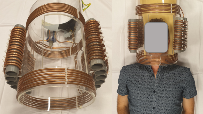
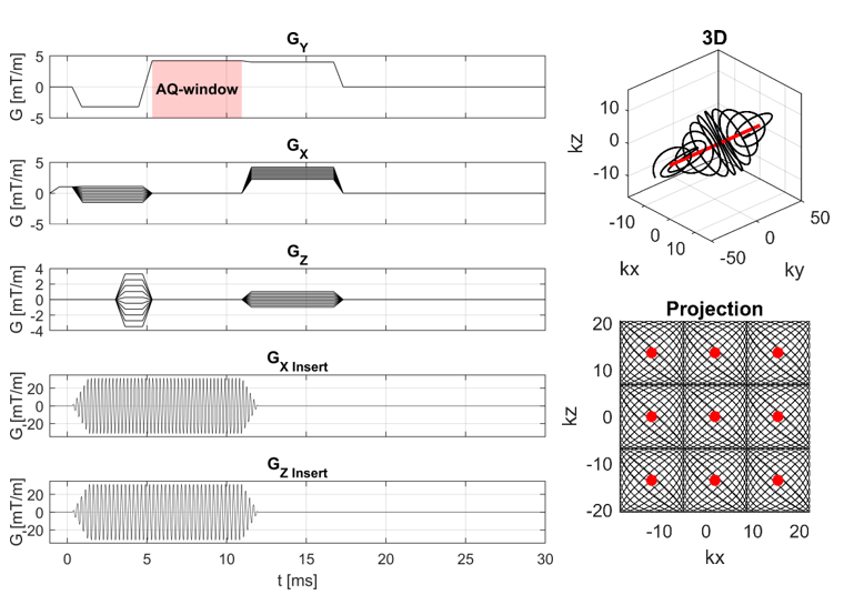
A dual-axis gradient insert was designed and produced in-house (Figure 1). The resulting setup featured an x-and z-axis, which were made resonant at 22.0 kHz (x) and 19.9 kHz (z) using capacitors. A two-channel audio amplifier (18 kW) was used to drive both axes, so far without gradient filters. Two external waveform generators synthesized the gradient waveforms and were triggered by a TTL-pulse send out by our 7T MR-system (Philips Achieva). A dynamic field camera (Skope) setup was used to measure the achievable gradient amplitudes.5 An 8-channel dipole array was added for RF transmit and receive.A modified 3D gradient-echo sequence was used for image acquisition. This sequence consisted of a readout gradient in one direction with concurrent oscillating gradient on the other two physical axes. Here, the whole-body gradients (GX, GY, GZ) were used in synergy with the gradient insert (GX,insert, GZ,insert). The frequency difference between the two oscillating gradient axes resulted in a Lissajous-like k-space trajectory, filling a cuboid in k-space at each TR as measured by the field cameras (Figure 2).
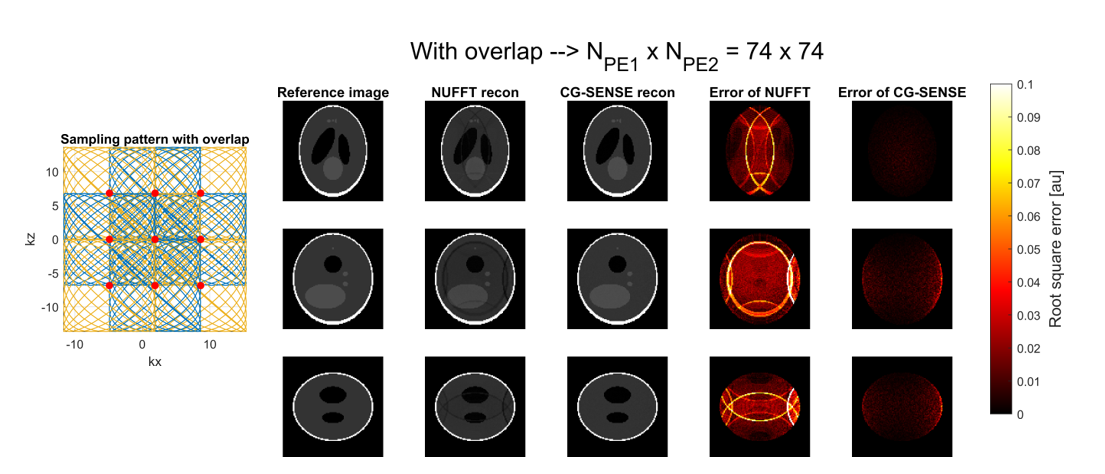
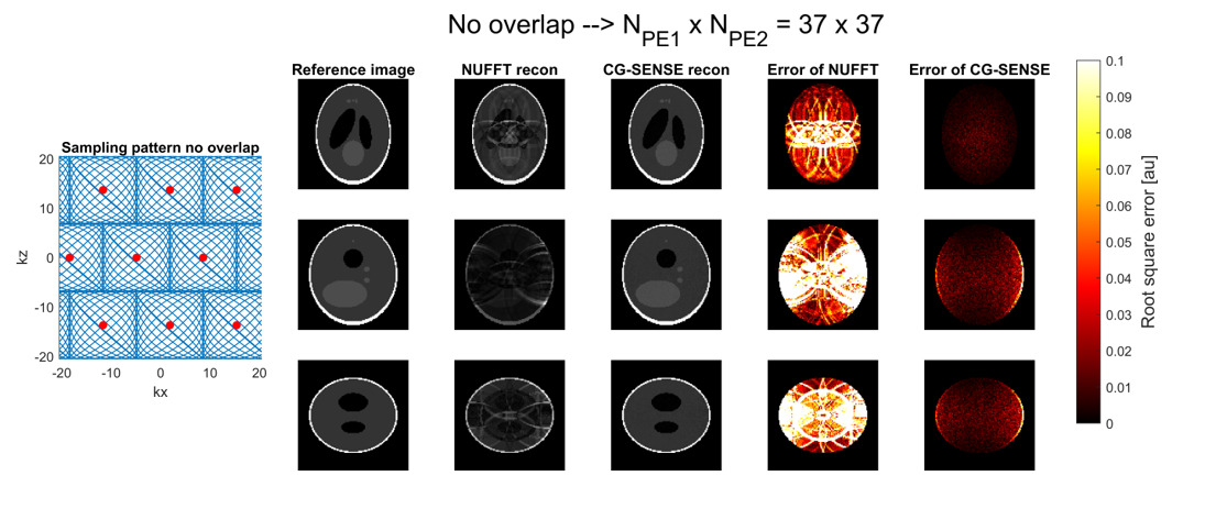
The imaging result of this sequence was simulated using a 3D Shepp-Logan phantom, a coil array of 16 channels (two rows of 8 channels), a 112x112x112 matrix size, and by using a generalized conjugate gradient (CG) SENSE reconstruction. Two cases were considered: one sequence which featured an overlap in the k-space sampling and one without overlap (see Figures 3 and 4). An SNR of 15 was imposed on the signal.
The aforementioned setup and sequence were used to image a water-filled phantom. This acquisition featured overlap in the k-space sampling and the following imaging parameters: FOV = 224x224x112 mm3, voxel size = 2 mm isotropic, TR/TE = 61/8.1 ms and flip angle = 25 degrees. Reconstruction was performed using a Non-Uniform Fast Fourier Transform (NUFFT) (CG-SENSE recon was not yet possible due to unavailable coil sensitivity data).
Results and Discussion
The gradient amplitude was measured to be 22.2 mT/m (@22 kHz) for the x-gradient and 20.8 mT/m (@19.9 kHz) for the z-gradient. Figures 3 and 4 show the results of the simulated imaging experiments using these measured amplitudes. Here, the NUFFT reconstruction showed aliasing artifacts while no artifacts were visible in the CG-SENSE reconstruction (see 2nd and 3rd column Figures 3 and 4).The reconstruction errors of both methods showed the same behavior as the images. Here, the residual of the CG-SENSE reconstruction featured unstructured noise, while the NUFFT reconstruction showed structural patterns from the aliasing (see 4th column Figure 3 and 4). Removing the overlap increased the noise in the images (see 5th column Figures 3 and 4), because of the reduced number of samples used for reconstruction.
In terms of acceleration, the simulations showed that artifact free images could be reconstructed when using only 37x37 = 1369 phase encoding steps. This equates to an acceleration factor of (112*112)/(37*37) = 9.1 when compared to the fully sampled image. Note, that the acceleration potential of this setup is limited by the amplitude of the oscillating gradient and can be increased by having separate amplifiers for each axis. In a recent report, a single-axis with one amplifier was able to produce gradient amplitudes reaching 40 mT/m.4
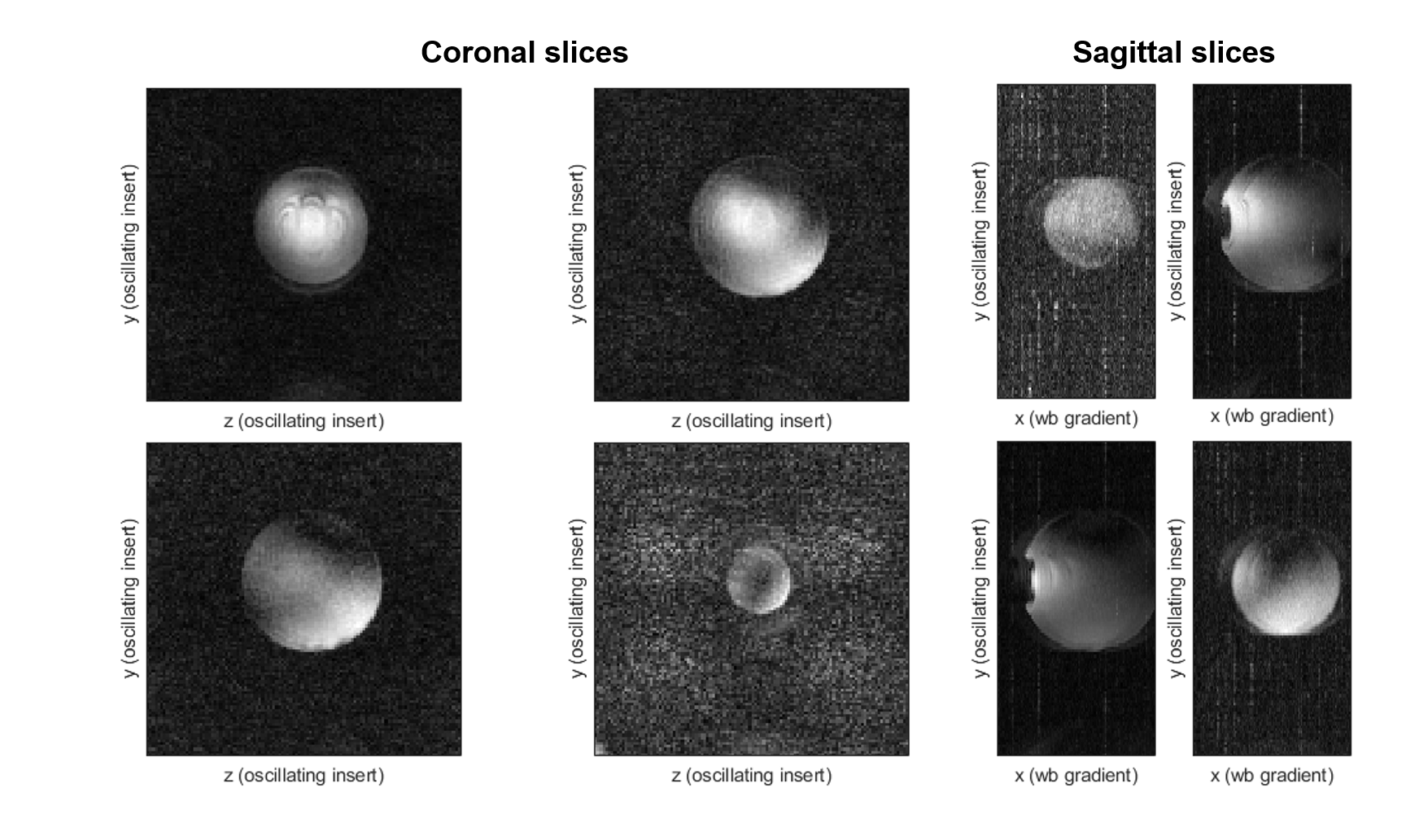
Figure 5 shows multiple slices through the water-filled phantom. Here, we see that almost no aliasing artifacts were visible in the coronal slices. Residual aliasing was visible in the sagittal slices as the NUFFT reconstruction cannot unfold the aliasing pattern from the oscillating gradients without coil sensitivity data. A CG-SENSE reconstruction, as was used in the simulation, could then be used to eliminate these artifacts. The noise in the images stemmed from an open RF-cage caused by the gradient inserts cable routing.
The presented setup did produce an audible sound at a beat frequency of 2.1 kHz when both axes were driven simultaneously. A completely silent dual axes setup may be achieved by embedding the coils in epoxy or retuning the dual axis setup with different capacitor values to decrease the frequency difference to an inaudible frequency.
Conclusion
We have demonstrated a setup for spatial encoding of 3D-MRI using two rapidly oscillating gradient axes driven around 20 kHz. The acceleration potential of this setup was simulated and found to be a factor of 9. First imaging experiments showed that imaging with such a setup is feasible.Acknowledgements
No acknowledgement found.References
1. Bilgic B, Gagoski BA, Cauley SF, et al. Wave-CAIPI for Highly Accelerated 3D Imaging. doi: 10.1002/mrm.25347.
2. Moriguchi H, Duerk JL. Bunched Phase Encoding (BPE): A New Fast Data Acquisition Method in MRI. Magn. Reson. Med. 2006;55:633–648 doi: 10.1002/mrm.20819.
3. Dispenza NL, Littin S, Zaitsev M, Constable RT, Galiana G. Clinical Potential of a New Approach to MRI Acceleration. Sci. Rep. 2019;9:1912 doi: 10.1038/s41598-018-36802-5.
4. Versteeg E, Klomp DWJ, Siero JCW. (2019), Supersonic imaging with a silent gradient axis driven at 20 kHz, #4586
5. Dietrich BE, Brunner DO, Wilm BJ, et al. A field camera for MR sequence monitoring and system analysis. Magn. Reson. Med. 2016;75:1831–1840 doi: 10.1002/mrm.25770.
Figures