Introduction

Non-uniform B₁⁺ at ultra-high field creates zones of signal dropout for brain imaging (temporal lobes, cerebellum) and non-uniform contrast weighting. In regions with little B₁⁺ sensitivity, small lesions may be hard to detect and the temporal SNR, which is a key metric in functional MRI, may be very low.
Parallel transmission (pTx) is a solution to this problem, but its adoption is hampered by complex engineering and safety (SAR) considerations as well as lengthy pre-scan and pulse computation steps^1,2.
Recently, a generalization of kT points and spoke pulses, commonly used in pTx, was proposed that uses a single transmit channel (birdcage coil) and a multiplicity of independently-driven shim loops positioned close to the head³. The “gradient blips” in spokes and kT point pulses are replaced by general, non-linear field variations between the RF pulses that are created by the shim array, and which are complementary to the B₁⁺ field profile.
Here, we propose a generalization of this shim-array strategy, whereby the RF and shim currents are played concurrently to yield uniform 3D flip-angle (FA) excitations.

Methods

Shim array: We use a 7T shim array with 31 loops supporting both RF and DC current (“AC/DC” coil) patterned on a close-fitting helmet. The B₀-field maps (Hz/Amp) of all channels ($$$B_0^{(s)}(\mathbf{r})$$$ in (2)) were measured in lengthy scans in a silicone-oil phantom using the vendor-provided field-mapping sequence (2-mm iso., dual-echo, $$$\Delta$$$TE=1.02ms). These maps are independent of the load and need to be acquired only once. RF transmission is by the birdcage coil.

Optimal control (OC): Each map was used as input in the "blOCh"-optimization framework^1,4. The target is a complete transfer of $$$M_z$$$ to $$$M_x$$$. The cost function is:
$$\bar{J}=J+\int_0^T(\mathbf{L}(\mathbf{r},t))^\mathrm{T}\{\mathbf{\Omega}(\mathbf{r},t)\mathbf{M}(\mathbf{r},t)-\dot{\mathbf{M}}(\mathbf{r},t)\}dt\,\,\,\,\,(1)$$
where the dynamical constraint of the Bloch equation (ignoring relaxation) is $$$\dot{\mathbf{M}}(\mathbf{r},t)=\mathbf{\Omega}(\mathbf{r},t)\mathbf{M}(\mathbf{r},t)$$$, and $$$J$$$ is the efficiency of the transfer. See Ref.⁴ for deeper explanations. In OC parlance, the shim currents are controls acting simultaneously with the RF and $$$G_x,\,G_y\,\mathrm{and}\,G_z$$$ gradient controls ($$$\mathbf{G}$$$ in (2)). The shim controls appear in the Bloch equations next to $$$\mathbf{G}$$$ and other B₀-related terms:
$$\mathbf{\Omega}(\mathbf{r},t)=\left[\begin{matrix}0&\omega_z(\mathbf{r},t)&-\gamma\,B_{1,y}(\mathbf{r},t)\\-\omega_z(\mathbf{r},t)&0&\gamma\,B_{1,x}(\mathbf{r},t)\\\gamma\,B_{1,y}(\mathbf{r},t)&-\gamma\,B_{1,x}(\mathbf{r},t)&0\end{matrix}\right]\,\,\,\,\,(2)$$
where $$$\omega_z(\mathbf{r},t)=\gamma\mathbf{G}(t)\cdot\mathbf{r}+\gamma\Delta\,B_0(\mathbf{r})+2\pi\sum_{s=1}^{31}B_0^{(s)}(\mathbf{r})I^{(s)}(t)$$$. Following Refs.^1,4 one can compute the cost-function derivative with respect to the shim controls, $$$\partial \bar J/\partial I^{(s)}$$$, and implement it in the OC algorithm (L-BFGS¹). For speed, we used approximations of $$$\partial \bar{J}/\partial I^{(s)}$$$, which are comparable in accuracy to the exact gradients¹, and much faster to compute⁵. Maximum 1000 iterations and convergence tolerances of $$$1\cdot\,10^{-5}$$$ were set.

Pulse optimizations: We varied pulse durations from 0.5 to 6 ms (10-µs dwell-time). We performed three kinds of optimizations (for each pulse duration): "RF only", "RF+Gradients" and "RF+Shims". The "RF only" optimizations (started from random guesses), and was then seeded to "RF+Gradients" and "RF+Shims" optimizations. Additional "RF+Gradients" and "RF+Shims" started from random guesses were also performed. All pulses were compared to a simple rectangular excitation pulse, denoted "RF block pulse". Constraints were 500-V RF magnitude; 4-A shim current per channel and 40 mT/m magnitude and 200 T/m/s slewrate on gradients.

Results & Discussion

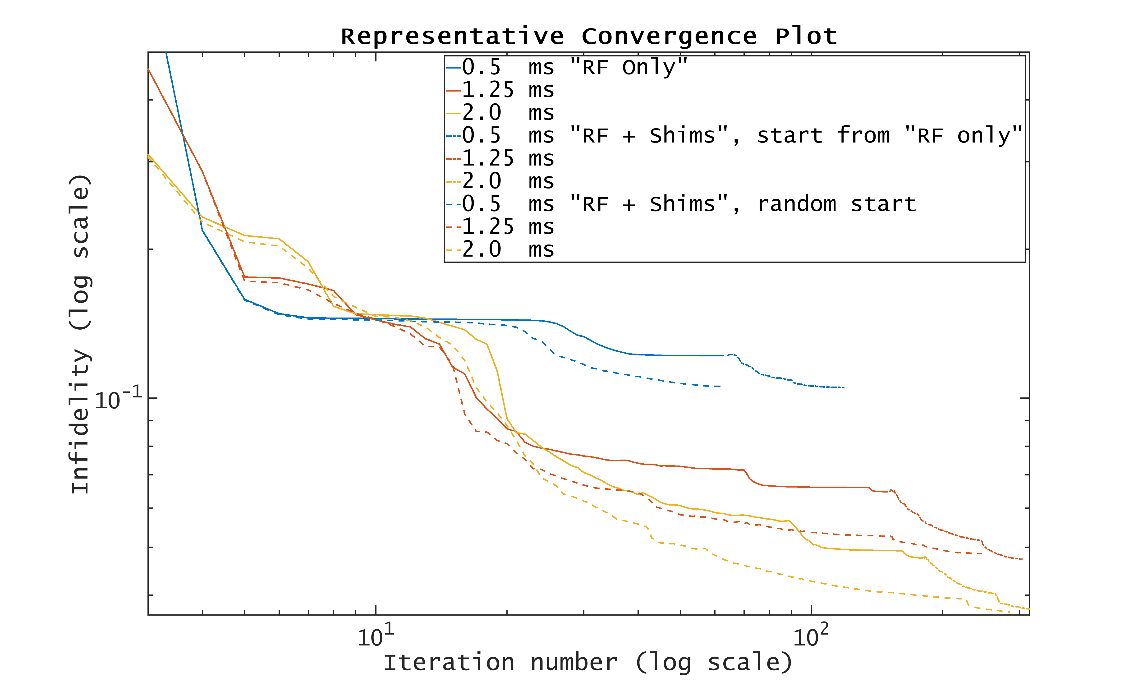
Figures 1a and 1b show 4-ms "RF+Shims" and "RF only" pulse solutions. Other pulses have similar appearance, except for the shortest pulses, which tend to be saturated in RF magnitude for most of the entire duration of the excitation. The shim waveforms shown in Figure 1c are representative of all pulse duration solutions. The waveforms are smoothly varying, which was not enforced in the OC framework, but is rather a characteristic of this kind of optimization. Figure 1d is a montage of the central slice of all the 31 shim sensitivity maps.
Figure 2 shows the infidelity convergence profiles of a representative subset of the "RF+Shims" and "RF only" optimizations.
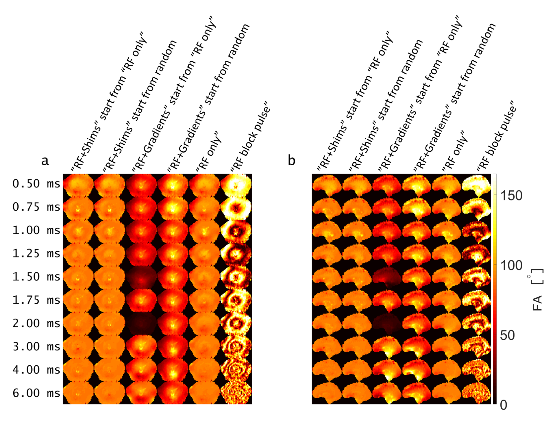
Figure 3a shows normalized root-mean-square errors (NRMSE) from the best iteration of each optimization strategy. The “RF+Shims” tend to produce better excitations using shorter durations than “RF only”. For example, the 1.25-ms "RF+Shims" pulses perform similarly (by NRMSE) as a 2-ms "RF only" pulse. Figure 3b shows that the "RF+Shims" tend to consume a little more average power than the "RF only" pulses of same durations, which is intuitive since the shim array currents dephase the magnetization in order to achieve more uniform excitations³. All optimized pulses roughly achieve the target FA (90°, Figure 3c&d) and the FA standard deviation decreases with pulse duration for all optimization strategies. Figure 4 shows some FA patterns from all pulses.
Our "RF+Gradients" optimizations were not successful. We could in 50% of cases observe an insignificant improvement starting from "RF only" for few iterations followed by rapid deterioration. This is likely due to the non-convex nature of the optimization problem, an issue that we will need to study in more detail in order to further improve the quality of our pulses.

Conclusion

We present an "RF+Shims" FA optimization strategy for uniform, 3D volume excitation, which extend the composite pulses of Rudrapatna et al.³ to continuous waveforms. Even using only modest current amplitudes (<4A/ch), the extra degrees of freedom provided by the shim array seem to be used advantageously by OC to reduce the pulse duration by ~38% for similar excitation quality at the cost of a minor increase in average RF power (~19%).

References

1. Vinding, M. S., Guérin, B., Vosegaard, T. & Nielsen, N. Chr. Local SAR, global SAR, and power-constrained large-flip-angle pulses with optimal control and virtual observation points. Magnetic Resonance in Medicine 77, 374–384 (2017).
2. Guérin, B., Gebhardt, M., Cauley, S., Adalsteinsson, E. & Wald, L. L. Local specific absorption rate (SAR), global SAR, transmitter power, and excitation accuracy trade-offs in low flip-angle parallel transmit pulse design: Low Flip-Angle Parallel Transmit Pulse Design. Magnetic Resonance in Medicine 71, 1446–1457 (2014).
3. Rudrapatna, U., Juchem, C., Nixon, T. W. & de Graaf, R. A. Dynamic multi‐coil tailored excitation for transmit B1 correction at 7 Tesla. Magnetic Resonance in Medicine 76, 83–93 (2016).
4. Vinding, M. S., Maximov, I. I., Tošner, Z. & Nielsen, N. Chr. Fast numerical design of spatial-selective rf pulses in MRI using Krotov and quasi-Newton based optimal control methods. The Journal of Chemical Physics 137, 054203 (2012).
5. Vinding, M. S. et al. (In preparation).