Introduction

In MRI, several types of RF that have different purposes (e.g., SLR, adiabatic, spin-lock) have been developed. Designing these pulses or developing the design rules requires a deep understanding of MR physics, and, therefore, is not easy. Recent advances in deep reinforcement learning (DRL) have demonstrated that self-learning enables an artificial intelligence (AI) agent to master complex games (e.g., Go and StarCraft) by repetitively playing self-matches^1-3. Using a similar approach, Shin et al. recently demonstrated that an AI agent can design a multiband SLR RF pulse⁴. In this work, we further investigate the idea of machine-designed RF and demonstrate that an AI agent successfully designs a more complex RF pulse (adiabatic RF) that satisfies given design criteria. Different from Shin’s work, which finds the optimum binary combination, the new task is to determine RF amplitude and phase with no specific constraint (e.g., no SLR transformation). Therefore, it is substantially more challenging. We named this novel design method as “DeepRF”.

Methods

A non-selective inversion RF pulse that has immunity to B₁⁺ inhomogeneity is designed.
[Hyperbolic secant RF] For a conventional adiabatic pulse, a hyperbolic secant (HS) pulse⁵ is designed with the coverage of B₁ from 0.1 to 2.0 and off-resonance (Δω₀) from -100 Hz to 100 Hz⁶. After optimization, the parameters were set to be β = 4000 rad/sec, μ = 2.0, duration = 8 ms, and maximum amplitude = 0.2 Gauss.
[Machine-designed RF] We utilized DRL⁷ to self-learn an RF design by trial and error. In DRL, a neural-network agent performs a series of actions and receives a reward that corresponds to the actions. This process is repeated so that the agent finds the optimal series of actions that maximize the reward. In our design, the agent determines a series of amplitude and phase values to generate an RF pulse (Fig.1a). Then, a Bloch simulator evaluates the performance of the pulse and returns a reward to the agent. The reward is calculated as follows:$$1/(1+\frac{1}{NM}\sum_{B_1}\sum_{\triangle\omega_0}M_z(RF,B_1,\triangle\omega_0))^2$$where N (= 50) and M (= 20) refer to the numbers of B₁ and Δω₀, respectively, and M_z is the longitudinal magnetization. The same B₁ and Δω₀ ranges as in the HS pulse are applied.
For our agent, a recurrent neural network (RNN)⁸, which gets the previous RF value and current magnetization as the inputs and determines the next RF value (amplitude and phase) as the output, is utilized (Fig.1b). The use of RNN is important because the magnetization is determined not only by the current RF input but also by the previous magnetization (a hidden state). The recurrent memory module of RNN allows the agent to understand the cumulative effect of the applied RF.
To reduce the degree of freedom, the agent generates 16 RF values, which correspond to the former half of an RF pulse. Then, the latter half is determined by a time-reversal version of the former half, generating a mirrored magnetization behavior. The final 32 complex-valued time points are linearly interpolated to 128-time points (Fig.1c).
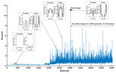
The process of generating and evaluating RF is continued until no better design is found for 2000 episodes (1 episode = 1 RF pulse). DeepRF had the same duration and maximum amplitude limit as the HS pulse.
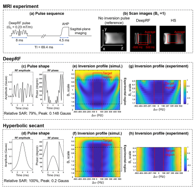
[Experiments] DeepRF and HS pulses were evaluated in a phantom (Fig.3a). A z-gradient (= 0.23 mT/m) was applied to introduce off-resonance. A sagittal plane was imaged at the nulling time (T₁ = 100 ms, TI = 69.4 ms and TR = 600 ms). The scan was repeated while scaling the reference voltage (= 0.5:0.1:1.7) to acquire the inversion efficiency profile. The profile was calculated by averaging central 80 lines normalized by a reference scan (Fig.3b). For comparison, computer-simulated profiles were generated.

Results

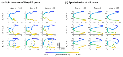
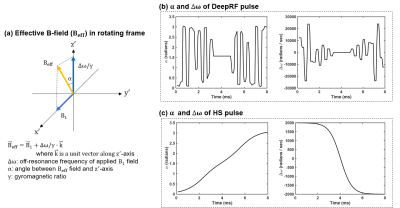
Figure 2 plots reward over episodes with a few example pulses. The final DeepRF pulse and HS pulse are shown in Figure 3c,d. The inversion efficiency plots of the simulation and experiment are presented in Fig 3e-h, showing good matches between the simulation and experiment. The DeepRF pulse has a smaller SAR (79% of HS) and lower peak amplitude (74% of HS). However, the inversion efficiency is degraded in low (< 0.4) and high (> 1.8) B₁. A few examples of spin behaviors during the pulse duration are plotted for different B₁ (0.7, 1.2, and 1.7) and Δω₀ (-100, 0, and 100 Hz) (Fig.4). Interestingly, the spin behaviors of DeepRF roughly are similar to the HS pulse when the B₁ scale is 0.7. However, it deviates for the higher B₁ scales, showing complex rapid motions. Furthermore, the effective field⁹ of DeepRF demonstrates rapid changes in both α and Δω, revealing a substantially different behavior to the well-known adiabatic principle (Fig.5)¹⁰.

Discussion and Conclusions

In this study, we proposed a novel RF design method, DeepRF, that utilized DRL to self-learn an RF design strategy. We demonstrated that DeepRF designs an inversion pulse robust to B₁ and off-resonance and suggested evidence for a different inversion pathway that is difficult to be predicted in the conventional adiabatic RF design. The current DeepRF pulse is limited to a non-selective inversion but the method can be extended to a slice-selective RF pulse.

Acknowledgements

This work was supported by the National Research Foundation of Korea (NRF) grant funded by the Korea government (MSIT) (NRF-2018R1A2B3008445), the Brain Korea 21 Plus Project in 2019, and Samsung Research Funding & Incubation Center of Samsung Electronics under Project Number SRFC-IT1801-09.