Introduction

Multiband RF pulses typically consist of several independent single-band RF pulses under the influence of a slice selective gradient. The utilization of multiple RF pulses leads to high peak and overall power when many bands are desired. For adiabatic RF pulses, the creation of multiple bands simultaneously is somewhat trickier due to the nonlinearity involved. Nonetheless, pulse summation still works, if certain power level constraints are met¹. More recently, it has been shown that multiband adiabatic inversion can be produced by periodically switching the gradients and RF on and off². This greatly reduces the power required but lengthens the pulse duration. Here, we present another technique for multiband adiabatic inversion using the concept of multiphoton excitation³. By oscillating the gradients, we can meet multiphoton resonance conditions at multiple locations, and thus achieve multiband multiphoton adiabatic inversions. Only a single adiabatic pulse is needed on the RF side.

Methods

Multiphoton excitation occurs whenever we satisfy the multiphoton resonance condition where integer multiples of multiple RF frequencies sum to equal the Larmor frequency and angular momentum is conserved. One form of multiphoton excitation in MRI occurs with a single photon polarized in the xy-plane ($$$B_{1,xy}$$$ with frequency $$$\omega_{xy}$$$) and one or more photons polarized along the z-axis ($$$B_{1,z}$$$ with frequency $$$\omega_{z}$$$). Since the magnetic fields of gradient coils in MRI are oriented along the z-axis, by oscillating gradients, we are able to provide z-axis photons for multiphoton resonances. As described previously³, the effective angular nutation frequency corresponding to an effective multiphoton amplitude for a single xy-photon and single z-frequency is
$$ \omega_{nut}=\gamma\ B_{1,xy}J_n\left(\frac{\gamma B_{1,z}}{\omega_z}\right) \hspace{2em} [1] $$
$$$J_n$$$ represents the Bessel function of the first kind of order $$$n$$$. $$$n$$$ represents the number of z-axis photons in the resonance. Note that $$$n$$$ can be positive or negative. For multiple z-frequencies, a Bessel function is multiplied for each frequency. For example, for two z-frequencies, we have resonances whenever
$$ \omega_{xy}=\gamma\ B_0+n\omega_{z1}+m\omega_{z2} \hspace{2em} [2] $$
and for each $$$n$$$ and $$$m$$$, the corresponding angular nutation frequency is given by
$$ \omega_{nut}=\gamma\ B_{1,xy}J_n\left(\frac{\gamma B_{1,z1}}{\omega_{z1}}\right)J_m\left(\frac{\gamma B_{1,z2}}{\omega_{z2}}\right) \hspace{2em} [3] $$
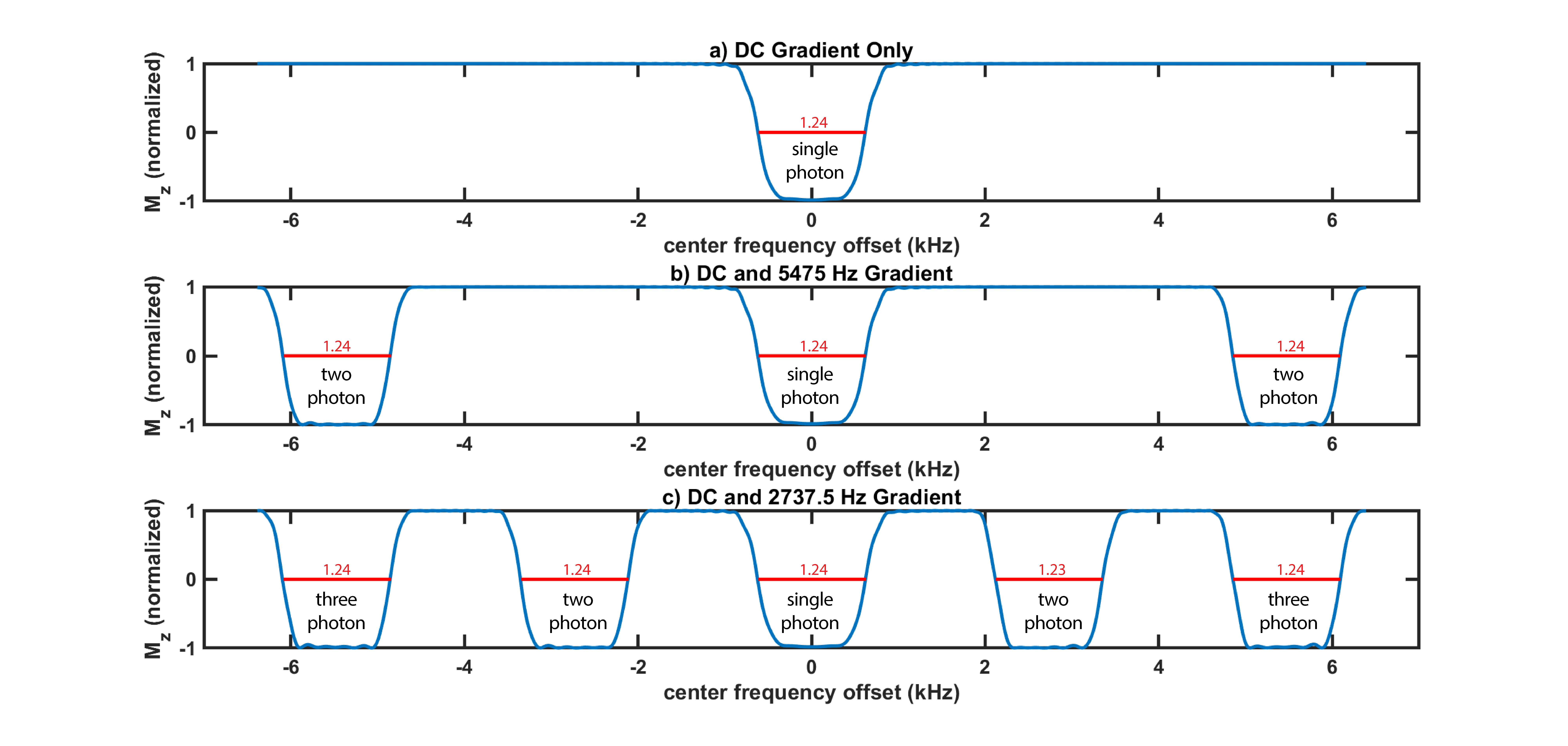
Therefore, if a constant DC gradient superimposes an oscillating AC gradient, given a frequency-centered $$$B_{1,xy}$$$, multiphoton resonances occur at locations where the local Larmor frequency (shifted by the DC gradient) and the frequency of the AC gradient satisfy Eq. [2]. Furthermore, in the case of a single gradient frequency, the argument to the Bessel function will be the ratio of the AC gradient strength to the DC gradient strength multiplied by the order of the Bessel function. Thus, if we choose the AC gradient strength to be 1.5 times the DC gradient strength, we will have excitation bands corresponding to an unscaled $$$B_{1,xy}$$$ at the center for the single-photon resonance, plus/minus $$$J_1(1.5)$$$ scaling for two photon resonances, plus/minus $$$J_2(3.0)$$$ scaling for three photon resonances, etc., until we are outside of the field of view. Note that this example provides a good choice for the AC gradient strength, as the Bessel functions are nearly maximized. Although we illustrate adiabatic excitation here, this scheme works for both adiabatic and non-adiabatic excitation.

Results

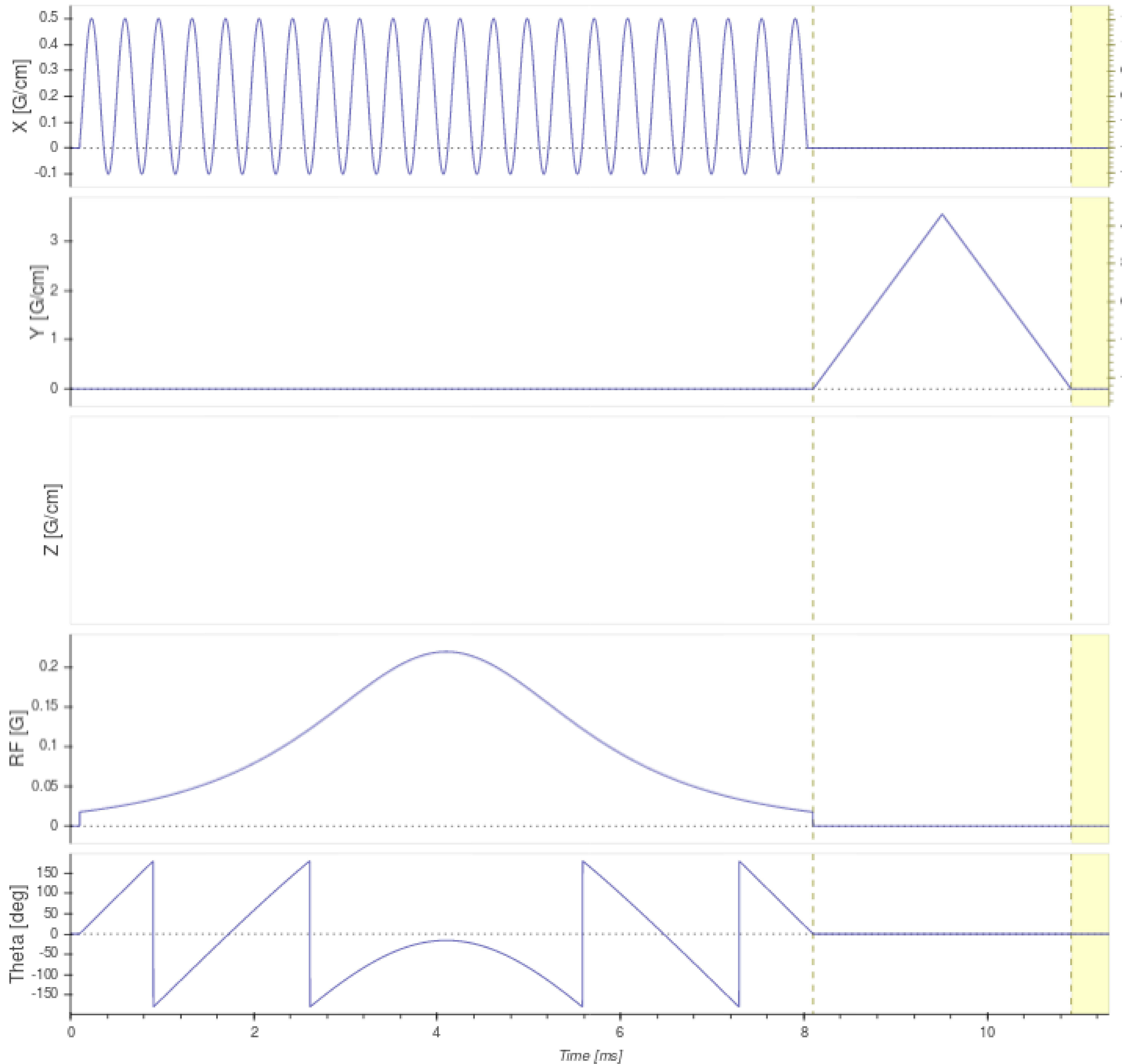
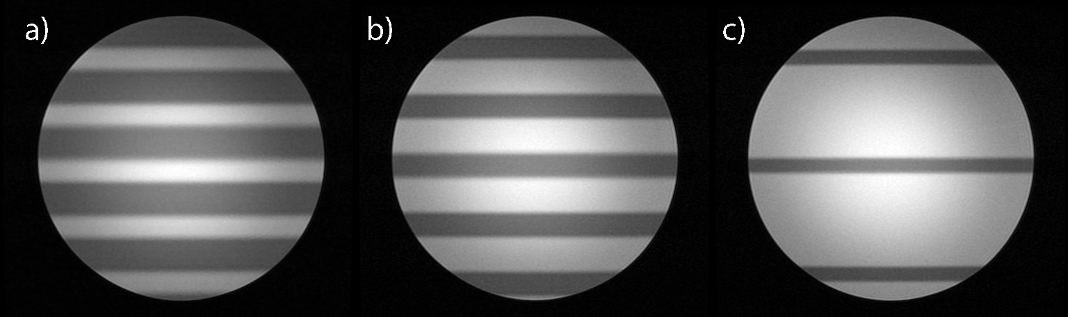
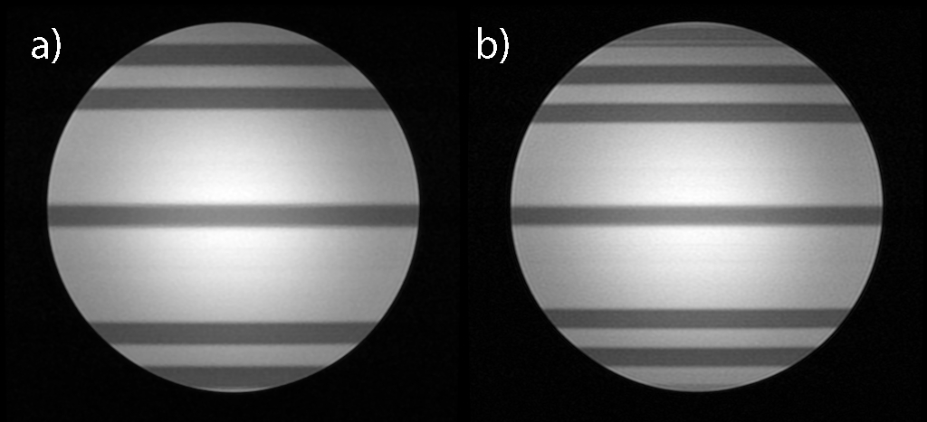
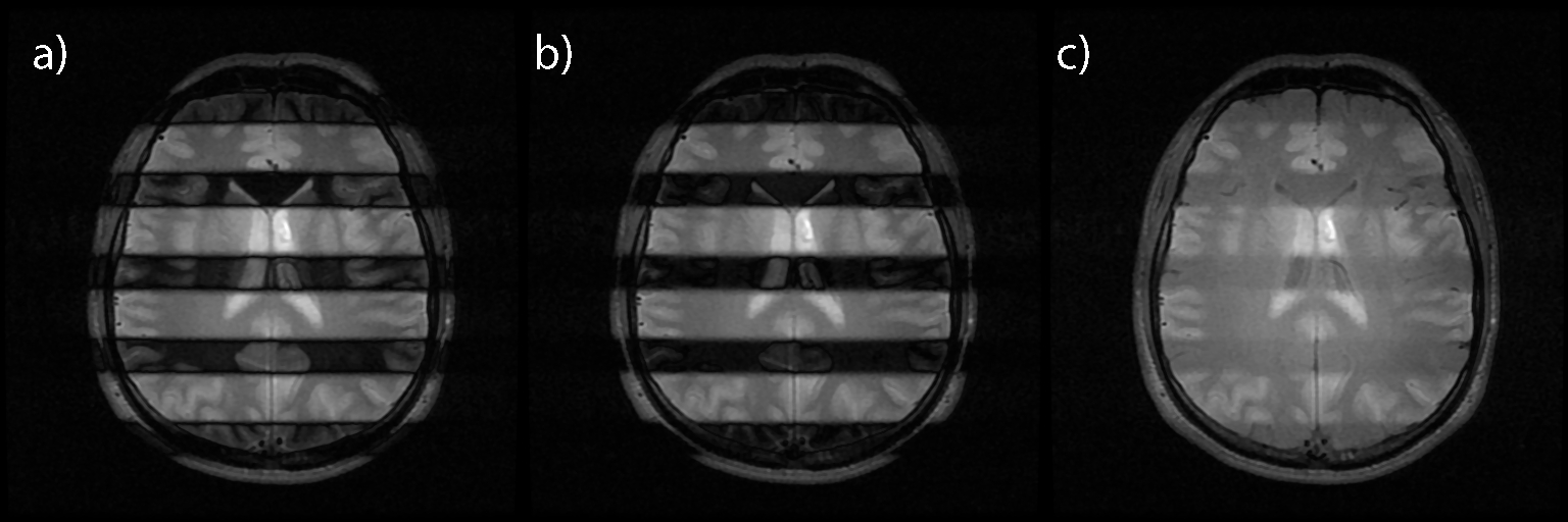
The proposed multiphoton multiband adiabatic inversion pulse was implemented in an inversion-recovery-prepared 2D fast spin echo sequence on a GE 3T MR750w scanner. The pulse sequence was coded using KSFoundation Epic⁴. To view the multiband inversion profiles, the inversion-pulse gradients were along an axis perpendicular to the fast spin echo imaging plane. Experiments were conducted on a spherical phantom and a human volunteer. Fig. 1 shows example pulse waveforms, Fig. 2 shows simulated resulting z-magnetization for the example pulses in Fig. 1 and others, Fig. 3 shows multiband inversion on a spherical phantom with various parameters, Fig. 4 shows an example of unevenly spaced inversion bands with multiple gradient frequencies, and Fig. 5 shows inversion bands over a human brain in vivo.

Discussion

When producing multiple inversion bands, the use of multiphoton resonances increases RF efficiency as the same RF pulse produces excitation in each band. The use of adiabatic pulses provides immunity against different effective pulse amplitudes of each multiphoton resonance, resulting in equal or comparable inversion. The RF pulse amplitude, however, needs to be high enough such that all the multiphoton resonances of interest fulfill the adiabatic condition. This leads to a slight increase in the RF pulse amplitude from a single-band adiabatic pulse as the Bessel functions are always less than or equal to 1. If some ripple is acceptable in the extra inversion bands, the RF pulse can be exactly the same as that of a standard single-band adiabatic pulse.

Conclusion

We have demonstrated power-efficient multiband adiabatic inversion pulses using the concept of multiphoton resonances. Such pulses may be useful for simultaneous multislice imaging techniques^5,6 or other more exotic pulse sequences that make use of adiabatic pulses⁷. This is one example demonstrating how a multiphoton interpretation of excitation can open new avenues for novel pulse design.

Acknowledgements

No acknowledgement found.