0569
Large-scale classification of breast MRI exams using deep convolutional networks
Shizhan Gong1, Matthew Muckley1, Nan Wu1, Taro Makino1, Gene Kim1, Laura Heacock1, Linda Moy1, Florian Knoll1, and Krzysztof Geras1
1New York University, New York, NY, United States
1New York University, New York, NY, United States
Synopsis
In this paper we trained an end-to-end classifier using a deep convolutional neural network on a large data set of 8632 3D MR exams. Our model can achieve an AUC of 0.8486 in identifying malignant cases on a test set reflecting the full spectrum of the patients who undergo the breast MRI examination. We studied the effect of the data set size and the effect of using different T1-weighted images in the series on the performance of our model. This work will serve as a guideline for optimizing future deep neural networks for breast MRI interpretation.
Purpose
In this work, we aim to build a deep learning based model to aid radiologists in breast MRI interpretation. Existing systems usually utilize a two-step approach, which initially determines the location and margins of the lesion, followed by classifying the extracted patches1-9. However, this lesion-level analysis may ignore some aspects of the data since most segmentation methods can only detect mass-type lesions. Additionally, lesion annotation is usually time-consuming and may introduce subjective biases. To overcome these limitations, we trained an end-to-end classifier using a supervised deep convolutional neural network directly on 3D MR images.Methods
We define the task of the breast MRI classification in the following manner. For each breast, we aim to predict two binary labels separately indicating the presence of malignant and benign findings.We use a novel neural network architecture called the Doubly Deep Convolutional Neural Network (see Figure 1). The input to the network is a 3D image, which is composed of several 2D slices. The network processes the input image in two stages. In the first stage, the input image is divided into several 2D slices, and each slice is fist processed separately. In the second stage, the outputs from the first stage are assembled into a 3D tensor on which a regular 3D CNN is applied.
The loss function we use to train our model has the following form:
$$\mathcal{L}\left(\{(\mathbf{x}^n, y^n_{L, B}, y^n_{L, M}, y^n_{R, B}, y^n_{R, M})\}_{n \in \{1,\ldots, N\}}\right) = -\frac{1}{N} \sum_{n=1}^{N} \sum_{s \in \{L,R\}} \sum_{c \in \{M,B\}}({y^n_{s,c}\log(\hat{y}_{s,c}(\mathbf{x}^n))+(1-y^n_{s,c})\log(1-\hat{y}_{s,c}(\mathbf{x}^n))})$$
where $$$M$$$ and $$$B$$$ stand for malignant and benign, $$$L$$$ and $$$R$$$ stand for left breast and right breast, $$$y^n_{s,c}$$$ represents whether the $$$n^{th}$$$ patient has a lesion of type $$$c$$$ in her breast $$$s$$$, and $$$\hat{y}_{s,c}(\mathbf{x}^n)$$$ represents the predicted probability of the corresponding label. We solve this learning task with multi-task learning in order to utilize information from benign cases to help learn the task of discriminating malignant cases.
Experimental Setup
Our study was IRB-approved and HIPAA-compliant. The data set is clinically realistic, containing 8632 MRI exams from 6295 patients scanned between 2008 and 2018 at a large academic institution. All women underwent bilateral breast DCE‐MRI using a 3.0T magnet (TimTrio, Siemens) or 1.5T magnet (Avanto, Siemens) in the prone position, using a 7 channel breast coil. The imaging protocol included both sagittal images and axial images. We collected fat-suppressed T1-weighted pre and three post-contrast acquisitions beginning 140 s - 760 s after the injection of a contrast agent (Magnevist or Gadavist). T1‐weighted imaging parameters included: repetition time / echo time (TR/TE) = (3.57-8.90)/(1.04-4.76) msec, flip angle 8°-20°, slice thickness 1 - 1.8 mm, matrix (320 - 480) $$$\times$$$ (182 – 388). There are four different T1-weighted images in the series for each exam, which were acquired at different time before (denoted by $$$\mathbf{x}_{t_0}$$$) or after (denoted by $$$\mathbf{x}_{t_1}$$$, $$$\mathbf{x}_{t_2}$$$ and $$$\mathbf{x}_{t_3}$$$) the injection of contrast agent. The target labels were derived from pathology reports. Figure 2 shows the distribution of target labels.The parameters of the network were learned using the Adam algorithm with a initial learning rate of $$$10^{-5}$$$. Our training data was augmented with random flips and crops of the original images, and no augmentations were applied during validation and testing. We trained the network for 50 epochs, allowing it to overfit, and picked the best model based on validation performance.Results
Our primary evaluation metric was the AUC. Our best model achieved an AUC of 0.8486 in identifying malignant cases on the test set. We evaluated predictions for both sides independently and pooled them to obtain one breast-level AUC, doing so for both the malignant and the benign lesion prediction tasks. We explored the relationship between data set size and test error when using the T1-weighted second post-contrast subtraction images. Figure 3 shows the classification performance improving as the number of training examples increases. Even with 100% of the data, the performance of the network has not yet saturated. We also explored the predictive value of different images in the series and their subtractions. Figure 4 shows the model trained on second post-contrast subtraction image has the best performance, which likely correlates to the greatest lesion conspicuity for lesions with plateau and wash-out temporal kinetics, which are more likely to be malignant11. We tried ensembling the classifiers trained in the previous section to further improve the performance. Following the approach of Caruana et al.12 we combined all seven models trained with different images in the series, resulting in the malignant AUC on the test set decreasing to 0.8459. These results show model ensembling brings us limited benefits.Discussion and Conclusion
In this paper, we showed our model was able to discriminate between benign and malignant lesions and achieved an AUC of 0.8486. These results set a strong baseline for future research on deep neural networks for classification of breast MRI exams. We show that performance of our neural network, although already strong, can be further improved by collecting more data. We also demonstrate a curious result showing the information in different T1-weighted images in the series appears almost completely redundant. Future work will investigate whether we can improve our method for aggregating information from different images in the series.Acknowledgements
The authors would like to thank Catriona C. Geras for correcting earlier versions of this manuscript, Marc Parente for help with importing the image data and Mario Videna and Abdul Khaja for supporting our computing environment. We also gratefully acknowledge the support of Nvidia Corporation with the donation of some of the GPUs used in this research. This work was supported in part by grants from the National Institutes of Health (R21CA225175 and P41EB017183).References
- Weijie Chen, Maryellen L Giger, and Ulrich Bick. A fuzzy c-means (fcm)- based approach for computerized segmentation of breast lesions in dynamic contrast-enhanced mr images. Academic Radiology, 13(1):63–72, 2006.
- Ashirbani Saha, Michael R Harowicz, and Maciej A Mazurowski. Breast cancer MRI radiomics: An overview of algorithmic features and impact of inter-reader variability in annotating tumors. Medical Physics, 45(7):3076– 3085, 2018.
- Mehmet Ufuk Dalmı¸s, Suzan Vreemann, Thijs Kooi, Ritse M Mann, Nico Karssemeijer, and Albert Gubern-M´erida. Fully automated detection of breast cancer in screening MRI using convolutional neural networks. Journal of Medical Imaging, 5(1):014502, 2018.
- P Herent, B Schmauch, P Jehanno, O Dehaene, C Saillard, C Balleyguier, J Arfi-Rouche, and S J´egou. Detection and characterization of MRI breast lesions using deep learning. Diagnostic and Interventional Imaging, 2019.
- Ke Nie, Jeon-Hor Chen, J Yu Hon, Yong Chu, Orhan Nalcioglu, and MinYing Su. Quantitative analysis of lesion morphology and texture features for diagnostic prediction in breast MRI. Academic Radiology, 15(12):1513– 1525, 2008.
- Hongmin Cai, Yanxia Peng, Caiwen Ou, Minsheng Chen, and Li Li. Diagnosis of breast masses from dynamic contrast-enhanced and diffusionweighted MR: a machine learning approach. PloS One, 9(1):e87387, 2014.
- Zhiyong Pang, Dongmei Zhu, Dihu Chen, Li Li, and Yuanzhi Shao. A computer-aided diagnosis system for dynamic contrast-enhanced MR images based on level set segmentation and ReliefF feature selection. Computational and Mathematical Methods in Medicine, 2015, 2015.
- Natalia O Antropova, Hiroyuki Abe, and Maryellen L Giger. Use of clinical MRI maximum intensity projections for improved breast lesion classification with deep convolutional neural networks. Journal of Medical Imaging, 5(1):014503, 2018.
- Daniel Truhn, Simone Schrading, Christoph Haarburger, Hannah Schneider, Dorit Merhof, and Christiane Kuhl. Radiomic versus convolutional neural networks analysis for classification of contrast-enhancing lesions at multiparametric breast MRI. Radiology, 290(2):290–297, 2018.
- Kaiming He, Xiangyu Zhang, Shaoqing Ren, and Jian Sun. Deep residual learning for image recognition. In Proceedings of the IEEE Conference on Computer Vision and Pattern Recognition, 2016. 6
- Christiane Katharina Kuhl, Peter Mielcareck, Sven Klaschik, Claudia Leutner, Eva Wardelmann, Jurgen Gieseke, and Hans H Schild. Dynamic breast MR imaging: are signal intensity time course data useful for differential diagnosis of enhancing lesions? Radiology, 211(1):101–110, 1999.
- Rich Caruana, Alexandru Niculescu-Mizil, Geoff Crew, and Alex Ksikes. Ensemble selection from libraries of models. In Proceedings of the Twentyfirst International Conference on Machine Learning. ACM, 2004.
Figures
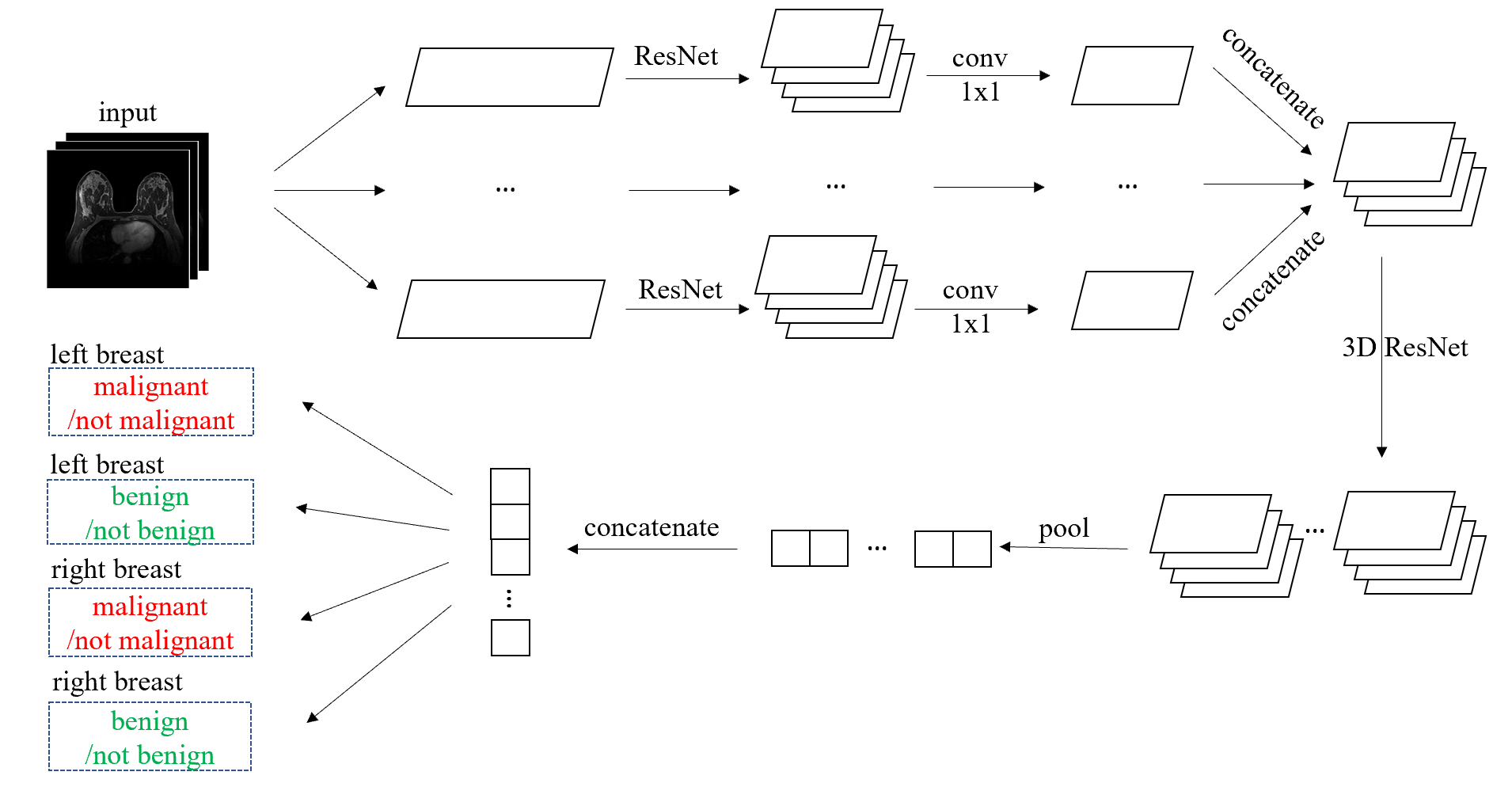
The Doubly Deep Convolutional Neural Network. The 2D ResNet is similar to ResNet-1810 without the global average pooling layer and the softmax layer, and the 3D ResNet consists of one 3D residual block with $$$3\times3\times3$$$ convolutional kernels and 128 output channels followed by a global maximum pooling layer and four separate softmax layers.
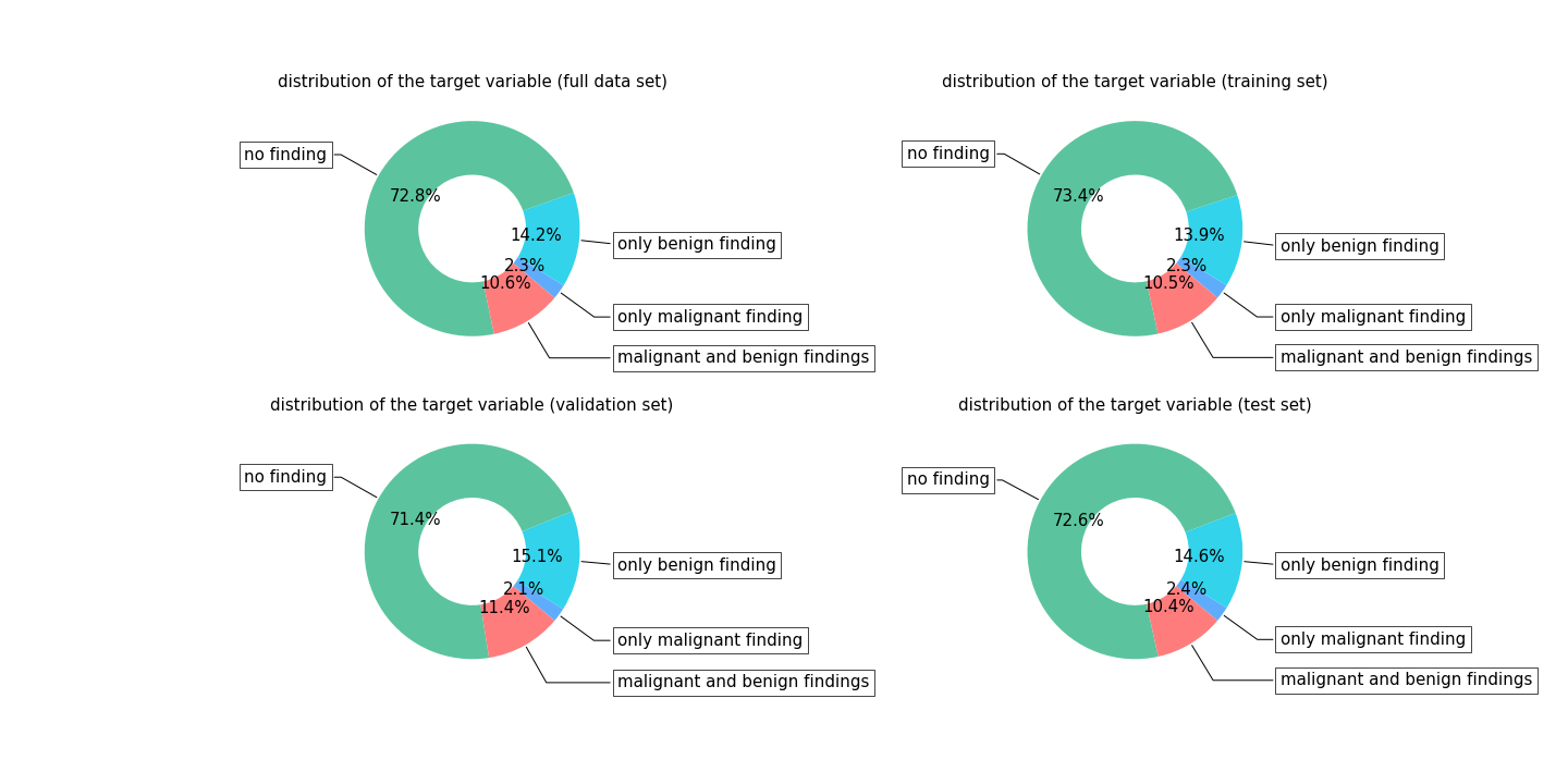
Distribution of target labels on each data set. We randomly divided the patients into training (3789 patients, 5192 exams), validation (1251 patients, 1704 exams) and test (1255 patients, 1736 exams) subsets.
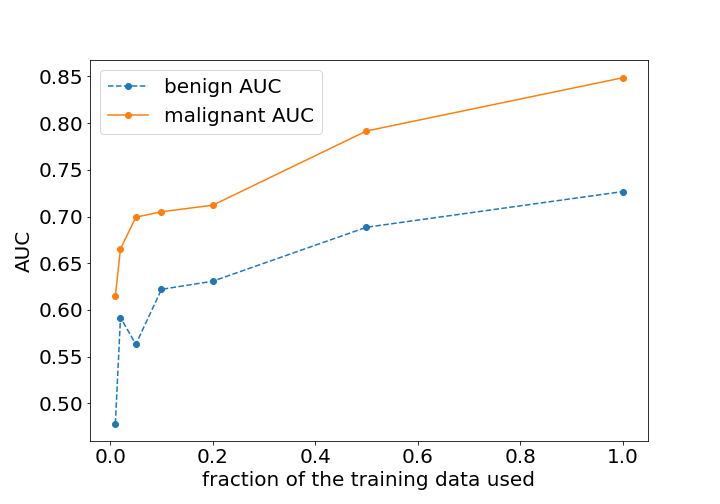
The effect of changing the fraction of the training data used on the performance on the test set. We trained separate networks on randomly sampled subsets of the full training set: 100%, 50%, 20%, 10%, 5%, 2% and 1% of the original training set.

The effect of different images in the sequence on the performance on the test set. We trained separate networks on the training sets composed of different images in the sequence and their subtraction.