0562
3D amplified MRI (aMRI) for visualizing pulsatile brain motion1Department of Electrical Engineering & Department of Structural Biology, Stanford University, Stanford, CA, United States, 2Department of Anatomy and Medical Imaging & Centre for Brain Research, University of Auckland, Auckland, New Zealand, 3Centre for Neuroscience Studies, Queen’s University, Kingston, ON, Canada, 4Department of Mechanical Engineering, Stevens Institute of Technology, Hoboken, NJ, United States, 5Centre for Advanced MRI, University of Auckland, Auckland, New Zealand, 6Translational and Molecular Imaging Institute, Icahn School of Medicine at Mount Sinai, New York, NY, United States, 7Department of Radiology, University of California, San Diego, CA, United States, 8Mātai Medical Research Institute, Gisborne-Tairāwhiti, New Zealand
Synopsis
Amplified Magnetic Resonance Imaging (aMRI) has been introduced as a new brain motion detection and visualization method. Originally employed to amplify pulsatile brain motion in 2D, aMRI has shown to be promising for differentiating abnormal from normal pulsatile brain motion in obstructive brain disorders. Here, we further improve aMRI with the introduction of a combined 3D aMRI acquisition and post-processing tool, with subsequent image processing with optical flow and strain mapping. The 3D aMRI tool is then tested on both multi-slice and volumetric data and its ability to capture 3D brain motion is analyzed.
Introduction
Amplified Magnetic Resonance Imaging (aMRI) has been introduced as a new brain motion detection and visualization method.1,2 aMRI been shown to be promising for differentiating abnormal from normal motion in Chiari Malformation patients;2 and for visualizing cerebrovascular motions (aFlow4). Using amplified strain maps, aMRI has also been shown to have relevance to concussion3. However, the original aMRI approach was a 2D post-processing algorithm which does not take into account motion in all three planes. Furthermore, it has only been applied to multi-slice data which typically only supports thick slices. Recently, a 3D aMRI post-processing algorithm has been introduced.5 Here, we further improve this approach with the introduction of a combined 3D aMRI acquisition and post-processing tool. The 3D aMRI acquisition is tested on both multi-slice and volumetric data and its ability to capture 3D brain motion is analyzed.Methods
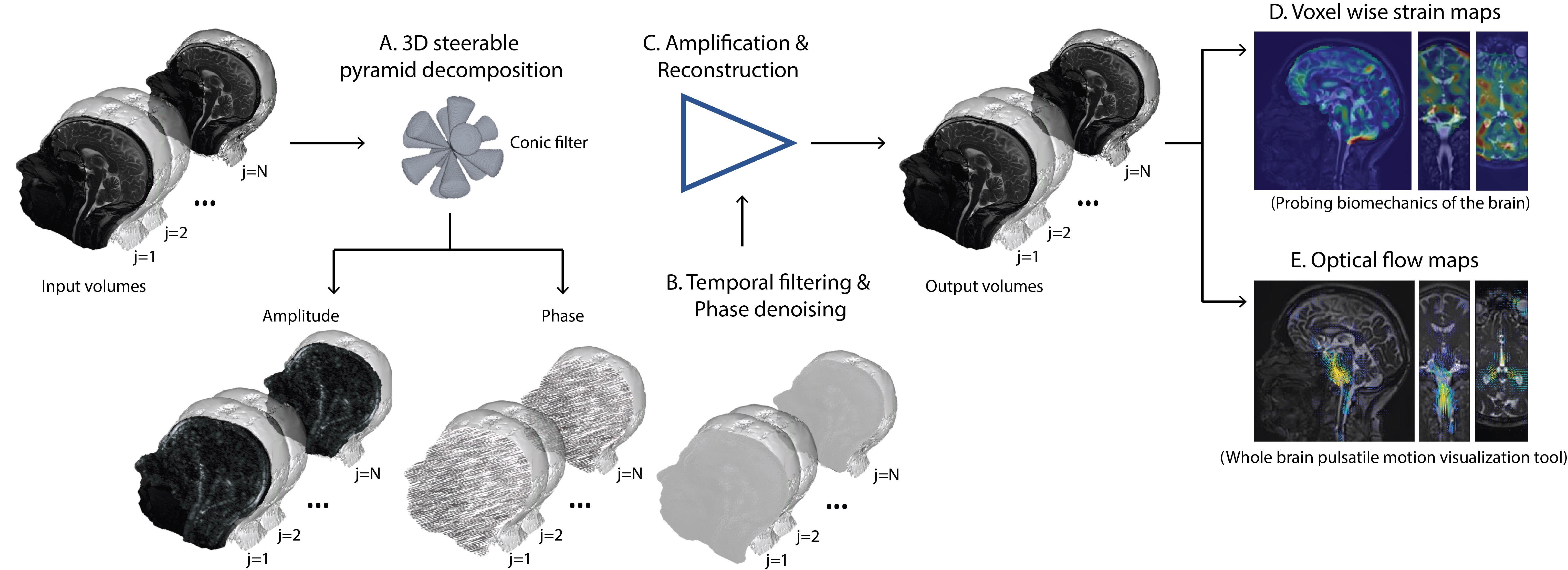
Image acquisition: Scans were performed on volunteers on a 3T MAGNETOM Skyra system (Siemens Healthcare, Erlangen, Germany) using a 32-channel head coil. Both multi-slice and 3D volumetric (true 3D) retrospectively cardiac-gated (cine) MRI datasets were acquired on a normal brain (adult volunteer 66yr/M). A balanced steady-state free precession (bSSFP) sequence acquired in the sagittal plane using peripheral pulse gating using the following parameters to target a common scan time of 2:40min and FOV of 23cm2. Parameters were as follows: matrix size = 1922, TR/TE/flip-angle=35ms/1.7ms/43°, acceleration factor = 2, #slices = 30, minimum achievable slice-thickness of 3mm (resolution = 1.2 x 1.2 x 3mm), and 25 cardiac phases. The 3D volumetric sequence used a matrix size = 2402, flip angle/TR/TE=50/1.7ms/26°, acceleration factor = 2, #slices = 64, partition-thickness of 1.2mm (resolution of 0.95 x 0.95 x 1.2mm), retrospective re-binning to 16 cardiac phases (the maximum achievable).Motion amplification: Fig. 1 illustrates the 3D aMRI method. With cine MRI images as input, 3D aMRI decomposes the volume images into scale and orientation using the 3D steerable pyramid.6,7,8 Here the spatial filters are 3D cones oriented along the six vertices of a cuboctahedron. The decomposition outputs an amplitude and phase value at each voxel. Amplification is achieved by temporally bandpass-filtering the phases, and multiplying them by a user-defined amplification factor of 15, and finally adding them to the original phase composites. This results in an exaggeration of the brain motion at different spatial scales and orientations. The volume is then reconstructed, resulting in a 4D movie with motion magnification within the desirable frequency range.
Image visualization: Strain maps were calculated as outlined in Champagne et al.3 Additionally, the Farnebäck optical flow method9 was applied to the aMRI data to help to visualize the distribution of apparent velocities. Optical flow estimates the brain’s displacement as a vector field, where displacement vectors are assigned to certain pixel positions that point to where those pixels are found in a successive frame.
Results & Discussion
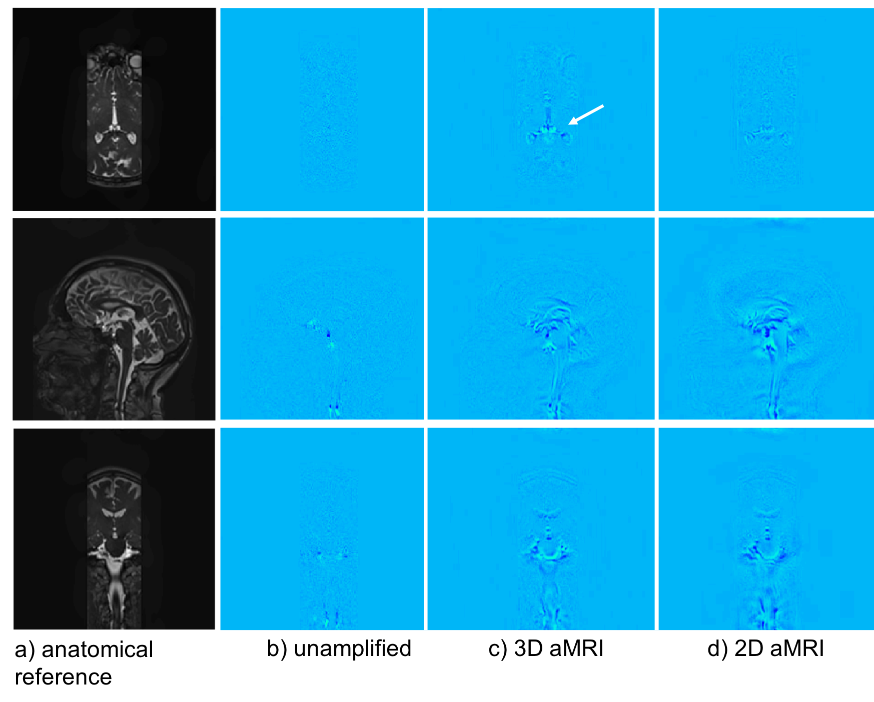
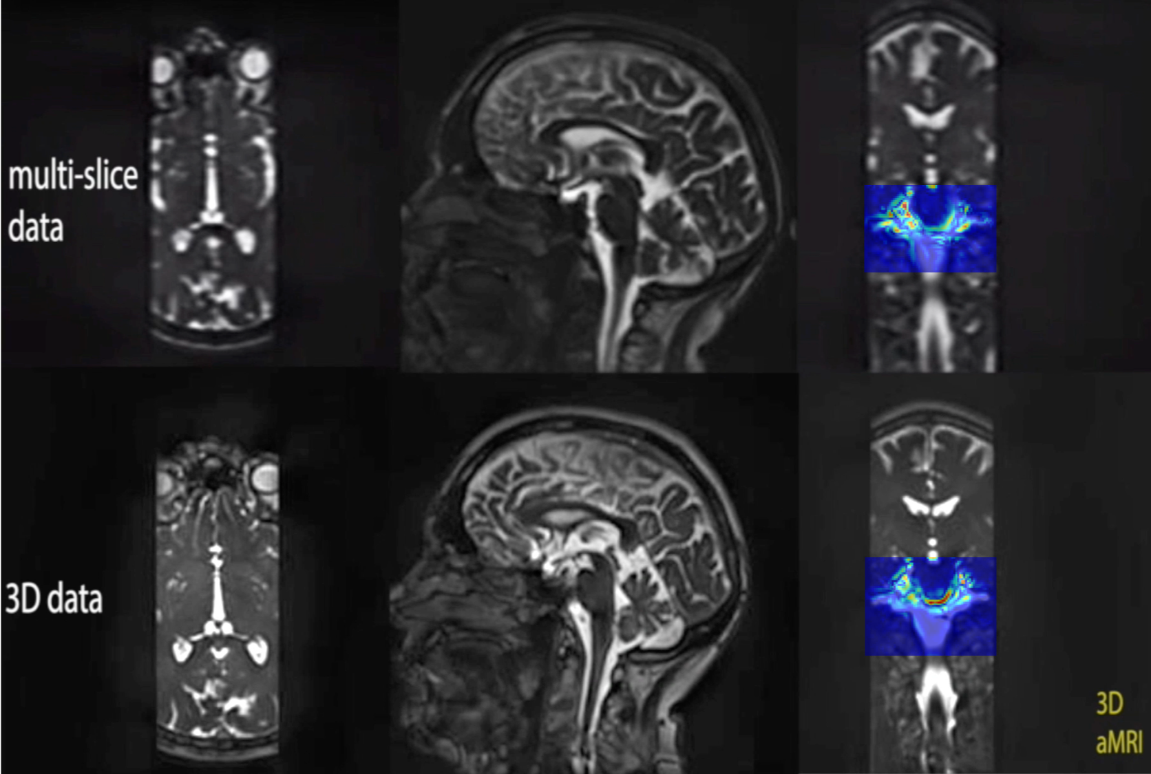
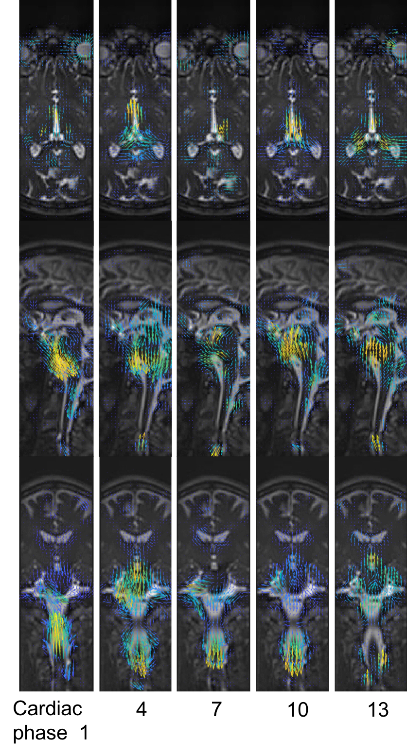
Fig. 2 depicts difference maps for both the 2D vs 3D aMRI algorithm applied on the volumetric data. Compared to the reference (unamplified) cine MRI, both 2D and 3D aMRI processing considerably enhanced the visualization of the pulsatile motion of the brain (shown www.stanford.edu/~iterem/Video_S1.mp4), particularly in the mid-brain region (as expected1,2). However, 3D aMRI has superior ability to capture motion compared with 2D aMRI, particularly reflected in the axial and coronal planes. Additionally, 3D aMRI shows an overall reduction in artifacts and superior pulsatile image quality. Since 2D aMRI only amplifies in-plane motion, artifacts are likely being introduced by the 2D algorithm itself. Strain maps produced from the 3D aMRI algorithm also depict the expected tissue strain in the ventricular region more reliably than 2D aMRI (Fig. 3). Multi-slice and 3D volumetric data processed with the 3D aMRI algorithm are shown www.stanford.edu/~iterem/Video_S2.mov, with the resolution advantage of volumetric data shown in Fig. 4. Finally, Fig. 5 shows optical flow maps of the pulsatile brain motion for the 3D aMRI (volumetric) dataset (video link www.stanford.edu/~iterem/Video_S3.mov). The physical change in shape of the ventricles by the relative movement of the surrounding tissues, and in particular the region of the basal ganglia, may be instrumental in propelling CSF from the lateral ventricles where it is formed, to the subarachnoid space. The motion within the tissue itself is seen to change direction during each cardiac cycle and may be instrumental in the process of driving extracellular fluid through the extracellular spaces.Conclusion
This study presents a new combined 3D aMRI acquisition and processing approach that enables more accurate visualization and quantification of human brain motion in all three planes. 3D aMRI was found to be particularly important for adequate visualization of motion in the axial and coronal plane. The application of this technique, coupled with visualization tools such as optical flow and strain mapping, may help us understand the dynamics of what drives the passage of CSF through the ventricular system, and the extracellular fluid within the brain tissue. This technique may open up exciting applications for a range of diseases and disorders that affect the biomechanics of the brain and brain fluids.Acknowledgements
Grant support and other assistance: National Institutes of Health (R21NS111415), University of Auckland FDRF strategic initiatives grant. We’d like to acknowledge Jonathan Richer, Michaela Schmidt, Toni Sinclair, and Kieran O’Brien from Siemens Healthineers for their tireless assistance with the 3D cine (a.k.a. 3D aMRI) acquisition. We are also grateful to Prof David Dubowitz for helpful discussions, and the Centre for Advanced MRI (CAMRI) technologists for their assistance with the scanning.
The * denotes equal authorship contribution.
References
- Holdsworth SJ, Salmani Rahimi M, Ni W, Zaharchuk G, Moseley ME. Amplified Magnetic Resonance Imaging (aMRI). Magn Reson Med. 2016;75(6):2245-54.
- Terem I, Ni W, Goubran M, Salmani Rahimi M, Zaharchuk G, Yeom KW, Moseley ME, Kurt M, Holdsworth SJ. Revealing sub-voxel motions of brain tissue using phase-based amplified MRI (aMRI). Magn Reson Med. 2018;80(6):2549-2559.
- Champagne A, Peponoulas E, Terem I, Ross A, Tayebi M, Chen Y, Coverdale N, Nielsen P, Wang A, Shim V, Holdsworth SJ, Cook D. Novel strain analysis informs about injury susceptibility of the corpus callosum to repeated impacts. Brain Communications, 2019
- Martinez J, Terem I, Holdsworth SJ, Kurt M. aFlow: A Novel Technique for Imaging Cerebrovascular Motions. Biomedical Engineering Society (BMES) Annual Meeting, Atlanta, U.S.A. 2018;3148.
- Abderezaei J, Martinez J, Terem I, Holdsworth SJ, Kurt M. Investigating the pulsatile motion of the brain through 3D phase-based amplified MRI. Imaging and Image Analysis for Biomechanics II for the 16th International Symposium on Computer Methods in Biomechanics and Biomedical Engineering and the 4th Conference on Imaging and Visualization (CMBBE), Columbia University, New York City, U.S.A, 2019;914.
- Wadhwa N, Rubinstein M, Durand F, Freeman WT. Phase-based video motion processing. ACM Trans Graph. Proceedings SIGGRAPH, 2013;32.
- Mathewson J, Hale D. Detection of channels in seismic images using the steerable pyramid. SEG Technical Program Expanded Abstracts: 2008;859-863.
- Luche CD, Denis D, Baskurt A. 3D steerable pyramid based on conic filters, Proc. SPIE, 2004;5266:260-268.
- Farnebäck G. Two-Frame Motion Estimation Based on Polynomial Expansion. 13th Scandinavian Conference on Image Analysis. Lecture Notes in Computer Science, (SCIA) 2003;2749:363-370.
Figures