0554
CSF Protein Cotent Estimation By T2 Component Analysis
Koichi Oshio1, Masao Yui2, Seiko Shimizu2, and Shinya Yamada3,4
1Department of Diagnostic Radiology, Keio University School of Medicine, Tokyo, Japan, 2Canon Medical Systems Corporation, Otawara-shi, Japan, 3Kugayama Hospital, Tokyo, Japan, 4Juntendo University, Tokyo, Japan
1Department of Diagnostic Radiology, Keio University School of Medicine, Tokyo, Japan, 2Canon Medical Systems Corporation, Otawara-shi, Japan, 3Kugayama Hospital, Tokyo, Japan, 4Juntendo University, Tokyo, Japan
Synopsis
Although there is no lymphatic system in the CNS, there seems to be a mechanism to remove macro molecules from the brain. CSF and ISF are thought to be parts of this pathway, but the details are not known. In this study, MR signal of the extracellular water, including CSF, was decomposed into components with distinct T2’s, to estimate content of macromolecules in each compartment. Assuming that protein content is relatively high along the clearance pathway, it might be possible to have some insight about this pathway from the obtained T2 map.
Inttroduction:
CSF (cerebrospinal fluid) and ISF (interstitial fluid) is thought to help large molecules to move out of the brain, but exactly how it is done is largely unknown. In the tissue other than the brain, this function is carried out by the lymphatic system. For example, drainage of labeled albumin injected in the brain into deep cervical nodes has been shown for rabbits (1). However, the lymphatic system itself is not present in the central nervous system, and some other pathway must be present to function in place of the lymphatic system. The information about this pathway may be obtained indirectly by analyzing T2 values of the brain tissue and CSF, assuming that T2 reflects the protein content of CSF / ISF. Since subarachnoid space has a complex shape, measuring T2 value for each pixel is not accurate due to partial volume effects. Also, in the brain parenchyma each pixel has different water compartments, each with different T2 values. In order to address this problem, the signal decay curve has to be decomposed into components with different T2 values. In this study, we used a method called non-negative least-squares (NNLS) for decomposition process.Methods:
1) MR imaging Total of four volunteers were enrolled with informed consent, after our IRB approval. Multi-echo images were acquired using a CPMG (Curr, Purcell, Meiboom, Gill) imaging sequence on a 3T clinical scanner (Canon Medical Systems). In order to reduce T1 contamination and signal oscillations, hard pulses were used as refocusing pulses. Therefore, only a single slice can be acquired at a time. Imaging parameters were as follows: TR = 5000 msec, the echo interval was 40 msec, slice thickness = 4mm, number of echoes was 25, TE = 40, 80, 120, ..., 1000 msec. 2) NNLS The decaying signal was decomposed into 25 T2 components, using NNLS, for each pixel. T2 values of 60 to 2000 msec, divided into 25 numbers with constant ratio interval were used. Standard Lawson and Hanson algorithm was used (2). 3) Color map After NNLS, each pixel has multiple T2 values. In order to display this information in understandable way for human eyes, a color map image was generated from the set of images for different T2 values. First, different color was assigned to each T2 component. Then, the RGB value for each point was added for all T2 components. By doing this it is possible to grasp overlapping T2 values, although it is not exactly quantitative.Results and discussion:
Acquired multi-echo images are shown on Fig. 1a. Using the NNLS, these echoes were decomposed into 25 components (Fig. 1b). T2 components of several selected pixels are shown on Fig. 2. Color map images were created for each slice from the T2 map (Fig. 3). As it can be seen in Fig. 1b, signal from intra-cellular component is dominant over extra-cellular water signal. In order to visualize the extra-cellular component more clearly, intra-cellular components, with T2 of around 60 msec, were assigned black color. The components with longer T2 (> 80msec) were assigned colors ranging from red to blue. In general, the CSF has longest T2 of around 1800 msec (blue), and the interstitial fluid has shorter T2, around 200 msec (red). Local distribution of interstitial fluid (ISF) roughly coincides with the white matter fibers. Other places in which ISF is seen include surface of the cortical gray matter, surface of the ventricles, choroid plexus, and around the blood vessels within the sub-arachnoid space. T2 value of 200 msec of the extracellular water roughly corresponds to 0.6 mM of protein, assuming the relaxivity of protein is about 7.6 mM-1s-1 (3). In the classical view, the CSF is formed at the choroid plexus, flows through the ventricles and the subarachnoid space, and is finally absorbed at the arachnoid villi into the venous sinus. However, many contradictory data have been shown in the past literature (4, 5), although alternative theory has not been established yet. From our results, assuming the T2 values are related to protein or large molecule content of the CSF / ISF, it is possible to obtain some insight into this removal pathway, by following a principle that extracellular water (ISF and CSF) exist continuously along the pathway, and the T2 value of the water is continuous, or changes slowly along the pathway. Based on this principle, we can identify some pathways as candidate for the “lymphatic” flow within the CNS.Conclusion:
A novel method to estimate T2 components of CSF and ISF without partial volume effect was developed. By separating T2 decaying curves into different T2 components, different kind of water compartments can be visualized without partial volume effects. Based on the color map indicating the distribution of extracellular water and its T2, it is possible to obtain some insight into pathway to transport large molecules in the central nervous system, where no lymphatic system is present.Acknowledgements
No acknowledgement found.References
- Yamada S, DePasquale M, Patlak CS, Cserr HF, Albumin Outflow into Deep Cervical Lymph from Different Regions of Rabbit Brain, Am J Physiol 1991; 261: H1197-1204.
- Bro R, de Jong S, A fast non-negativity-constrained least squares algorithm, J Chemometrics 1997; 11: 393-401.
- Daoust A, Dodd S, Nair G, Bouraoud N, Jacobson S, Walbridge S, Reigh DS, Koretsky A, Transverse relaxation of cerebrospinal fluid depends on glucose concentration, Magn Reson Imaging 2017; 44: 72-81.
- Hassin GB, Oldberg E, Tinsley M, Changes in the brain in plexectomized dogs: with comments on the cerebrospinal fluid, Arch Neurol Psychiatr 1937; 38: 1224-1239.
- Kudo K, Harada T, Kameda H, Uwano I, Yamashita F, Higuchi S, Yoshioka K, Sasaki M, Indirect proton MR imaging and kinetic analysis of 17O-labeled water tracer in the brain, Magn Reson Med Sci 2018; 17: 223-230.
Figures
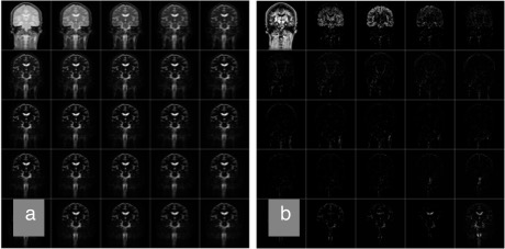
Acquired multi-TE images (a) and result of T2 decomposition (b). Images were acquired by a CPMG imaging sequence with echo interval of 40 msec, echo train length of 25. These images were decomposed into 25 T2 components, ranging from 60 msec to 2000 msec. On the figure, TE or T2 increases from left to right, then top to bottom.
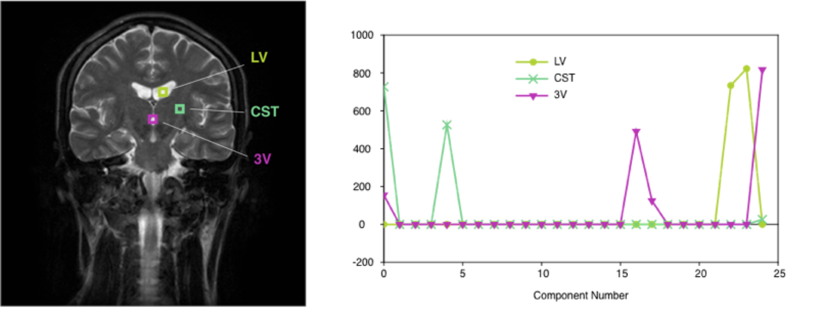
Example of the result of decomposition with brain images. Three pixels were selected as the example. In many pixels, T2 values are clustered into two or three groups. LV: lateral ventricle, CST: cortico-spinal tract, 3V: third ventricle.
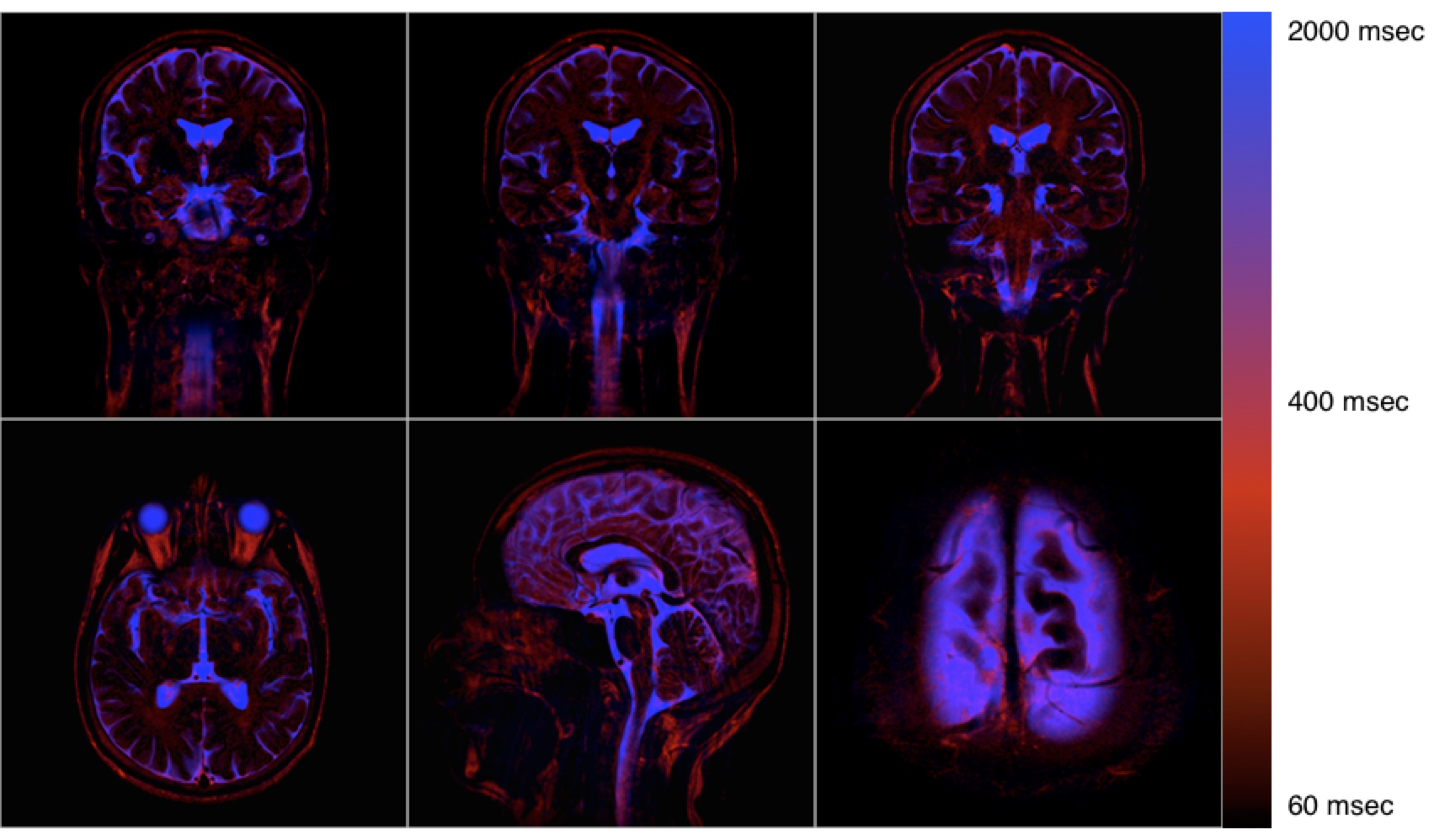
Typical color maps. Pixels are roughly divided into three groups: intra-cellular (black), extra-cellular (red), and the CSF (blue). The extracellular water is distributed in the white matter, the brain surface, dural side of subarachnoid space or possibly in the subdural space, choroid plexus, etc. The T2 of the fat tissue is close to that of extracellular water, and it is sometimes diffucult to distinguish these. The lower left image is an axial slice at the top of the head (magnified). In this image, fat saturation was turned on.