0531
Correlation Time as a New MRI Contrast
Hassaan Elsayed1,2, Jouni Karjalainen1,2, Nina Hänninen1,3, Isabel Stavenuiter3, Stefan Zbyn1,4, Mikko Nissi1,3, Miika T. Nieminen1,2,5, and Matti Hanni1,2,5
1Research Unit of Medical Imaging, Physics and Technology, University of Oulu, Oulu, Finland, 2Medical Research Center, University of Oulu and Oulu University Hospital, Oulu, Finland, 3Department of Applied Physics, University of Eastern Finland, Kuopio, Finland, 4Center for Magnetic Resonance Research, Department of Radiology, University of Minnesota, Minneapolis, MN, United States, 5Department of Diagnostic Radiology, Oulu University Hospital, Oulu, Finland
1Research Unit of Medical Imaging, Physics and Technology, University of Oulu, Oulu, Finland, 2Medical Research Center, University of Oulu and Oulu University Hospital, Oulu, Finland, 3Department of Applied Physics, University of Eastern Finland, Kuopio, Finland, 4Center for Magnetic Resonance Research, Department of Radiology, University of Minnesota, Minneapolis, MN, United States, 5Department of Diagnostic Radiology, Oulu University Hospital, Oulu, Finland
Synopsis
In this study, we determined correlation time ($$$\tau_c$$$ ), a parameter that we propose as MRI contrast indicative of the structure of articular cartilage. $$$T_{1\rho}$$$ dispersion data were acquired from intact patellar bovine cartilage samples and $$$\tau_c$$$ maps were obtained by fitting a Lorentzian model function to the $$$T_{1\rho}$$$ dispersion. The association between $$$\tau_c$$$ and the tissue properties was assessed by correlation analysis between $$$\tau_c$$$ and histology. The results suggest that the proposed parameter $$$\tau_c$$$ as well as other fitting parameters can reveal cartilage structure. More investigation is needed to establish correlation between $$$\tau_c$$$ and histology.
Introduction
Magnetic relaxation of nuclear spins is dependent on their local environment and the molecular processes they are involved in. The purpose of this study is to develop a new MRI contrast for the noninvasive evaluation of the cartilage macromolecular composition. Our aim is to estimate the apparent correlation time ($$$\tau_c$$$) of molecular processes in cartilage specimens using dispersion of the relaxation rate in the presence of spin-lock field, ($$$R_{1\rho} = 1/T_{1\rho}$$$).Methods
Bovine patellar osteochondral plugs ($$$N = 8$$$) were imaged using a 9.4 T scanner to obtain $$$T_2$$$-weighted images (TE = 10, 15, 23, 35, 54, 83 and 128 ms) as well as $$$T_{1\rho}$$$-weighted images (TSL= 0, 8, 16, 32, 64 and 128 ms) at 15 spin-locking amplitudes (SLA) from 200 to 5000 Hz.1 $$$T_2$$$ and $$$T_{1\rho}$$$ maps were obtained by fitting mono-exponential model to the corresponding weighted images. The following function was fitted to $$$R_{1\rho}$$$ dispersion pixel-by-pixel (Figure 1) to create $$$\tau_c$$$ maps:2,3$$R_{1\rho} = \frac{3A\tau_c}{1+16\pi^2f_1^2\tau_c^2} + B$$
where $$$\tau_c$$$, $$$A$$$ and $$$B$$$ are the fitting parameters and $$$f_1$$$ is the spin locking amplitude (Hz). Polarized light microscopy was used to measure retardation which is indicative of collagen anisotropy.4 Digital densitometry was used to measure optical density which is a measure of proteoglycan content.5
Regions of interest (ROIs) were cropped from all MRI and histology maps for statistical analysis. Spearman correlation analysis was used to estimate the association between MRI parameters: $$$\tau_c$$$, $$$A$$$, $$$B$$$, $$$T_2$$$ and $$$T_{1\rho}$$$ at 400 Hz, and reference parameters: retardation and optical density. The correlation was obtained from bulk values and zonal averages. Bulk value is the mean of the whole ROI, while zonal average is the mean of datapoints belonging to one cartilage zone: superficial, transitional or radial. MRI zones were defined visually from $$$T_2$$$ maps and histology zones were defined visually from the fibril angle profiles determined from polarized light microscopy. Correlation is identified as weak (0.3<r<0.5), moderate (0.5<r<0.7) or strong (r>0.7).
Results
Different MRI maps showed different structural information (Figure 2) as did the corresponding maps of the reference parameters (Figure 3). The $$$\tau_c$$$ maps showed a laminar appearance similar to $$$T_2$$$ and $$$T_{1\rho}$$$ maps. $$$\tau_c$$$ values were in the range of 100-250 µs in the superficial zone, 200-500 µs in the radial zone, and less than 100 µs in the transitional zone. $$$A$$$ maps also showed laminar appearance although different than $$$\tau_c$$$ appearance, while $$$B$$$ maps showed only minor changes along the depth of the cartilage. Retardation maps showed a laminar structure reciprocal to that of $$$T_2$$$, while the optical density values were increasing along the cartilage depth.Spearman correlation coefficients of $$$\tau_c$$$, $$$A$$$, $$$B$$$, $$$T_2$$$ and $$$T_{1\rho}$$$ at 400 Hz versus retardation and optical density from the bulk analysis varied from weak to moderate (Table 1). Moderate correlation was found between $$$B$$$ and optical density, while weak correlation was found between $$$\tau_c$$$ and retardation, $$$\tau_c$$$ and optical density, $$$A$$$ and optical density, and $$$T_2$$$ and optical density. None of the bulk correlations were statistically significant ($$$p < 0.05$$$).
Spearman correlation coefficients of $$$\tau_c$$$, $$$A$$$, $$$B$$$, $$$T_2$$$ and $$$T_{1\rho}$$$ at 400 Hz versus retardation and optical density from the zonal mean analysis ranged from weak to strong (Table 2). The analysis showed strong correlation between $$$T_2$$$ and retardation in the superficial zone. In the superficial zone, moderate correlation was found between $$$B$$$ and retardation as well as $$$T_2$$$ and optical density, while weak correlation was found between $$$B$$$ and optical density as well as $$$T_{1\rho}$$$ at 400 Hz and retardation. In the transitional zone, weak correlation was found between $$$A$$$ and retardation, $$$B$$$ and optical density, $$$T_2$$$ and optical density as well as $$$T_{1\rho}$$$ at 400 Hz and retardation. In the deep zone, weak correlation existed between $$$\tau_c$$$ and retardation, $$$A$$$ and optical density, $$$B$$$ and optical density, $$$T_{1\rho}$$$ at 400 Hz and retardation as well as $$$T_{1\rho}$$$ at 400 Hz and optical density. The correlation between $$$T_2$$$ and retardation in the superficial zone was the only statistically significant result in the zonal mean analysis.
Discussion
The parameters $$$\tau_c$$$, $$$A$$$ and $$$B$$$ provide a compact form to represent $$$T_{1\rho}$$$ relaxation on a wide range of spin-lock fields. The $$$\tau_c$$$ values we obtained are in agreement with the results obtained by Duvvuri et al. in bovine cartilage.6 It is thought that this range of correlation times is related to chemical exchange.6,7The new MRI parameters appear to provide similar information as histology. However, the low statistical power due to the small sample size discourages us from directly interpreting the contents of the MRI data via histology.
Conclusion
In this study we have represented the structure of articular cartilage with novel MRI contrasts: correlation time and two additional parameters $$$A$$$ and $$$B$$$. The parameters were obtained by fitting a Lorentzian model function to the $$$T_{1\rho}$$$ dispersion. We conclude that not only $$$\tau_c$$$ but also $$$A$$$ and $$$B$$$ can provide information on the structure of the cartilage. Although we see a promise in this approach for cartilage characterization, the relations between the new parameters and histology call for more investigation.Acknowledgements
We thank Henning Henschel and Marianne Haapea for their fruitful discussions.References
- Nissi MJ et al. (2018). Proc. Intl. Soc. Magn. Reson. Med 26:0197
- Hanni M et al. (2015). Proc. Intl. Soc. Magn. Reson. Med. 23:117
- Elsayed H et al. (2016). Proc. Intl. Soc. Magn. Reson. Med. 24:3003.
- Rieppo J et al. (2008). Microsc. Res. Tech. 71:279
- Király K et al. (1996). Histochem. J. 28:99
- Duvvuri U et al. (2002). Osteoathr Cartilage. 10:838.
- Gilani, IA et al. (2016). NMR Biomed. 29:841
Figures
Figure 1: Measured $$$R_{1\rho}$$$ dispersions and the corresponding model fits for three pixels representative of the different zones in articular cartilage.
Figure 2: The top row shows maps
of MRI parameters: $$$\tau_c$$$, $$$A$$$, $$$B$$$, $$$T_2$$$ and
$$$T_{1\rho}$$$ measured at 400 Hz (from left to right). The corresponding mean
profiles of each representative map are plotted in the bottom row.
Figure 3: Representative maps of
reference parameters: retardation (left) and optical density (middle) of the
same sample in Figure 4. The plot (right) shows mean profiles of both
parameters. Higher retardation reflects higher collagen anisotropy and vice versa, while higher optical density reflects higher proteoglycans content and vice versa.
Table 1: Spearman correlation
coefficients of MRI parameters: $$$\tau_c$$$, $$$A$$$, $$$B$$$, $$$T_2$$$ and
$$$T_{1\rho}$$$ at 400 Hz vs histological parameters: retardation and optical
density. The correlations are calculated from bulk mean values from all
samples.
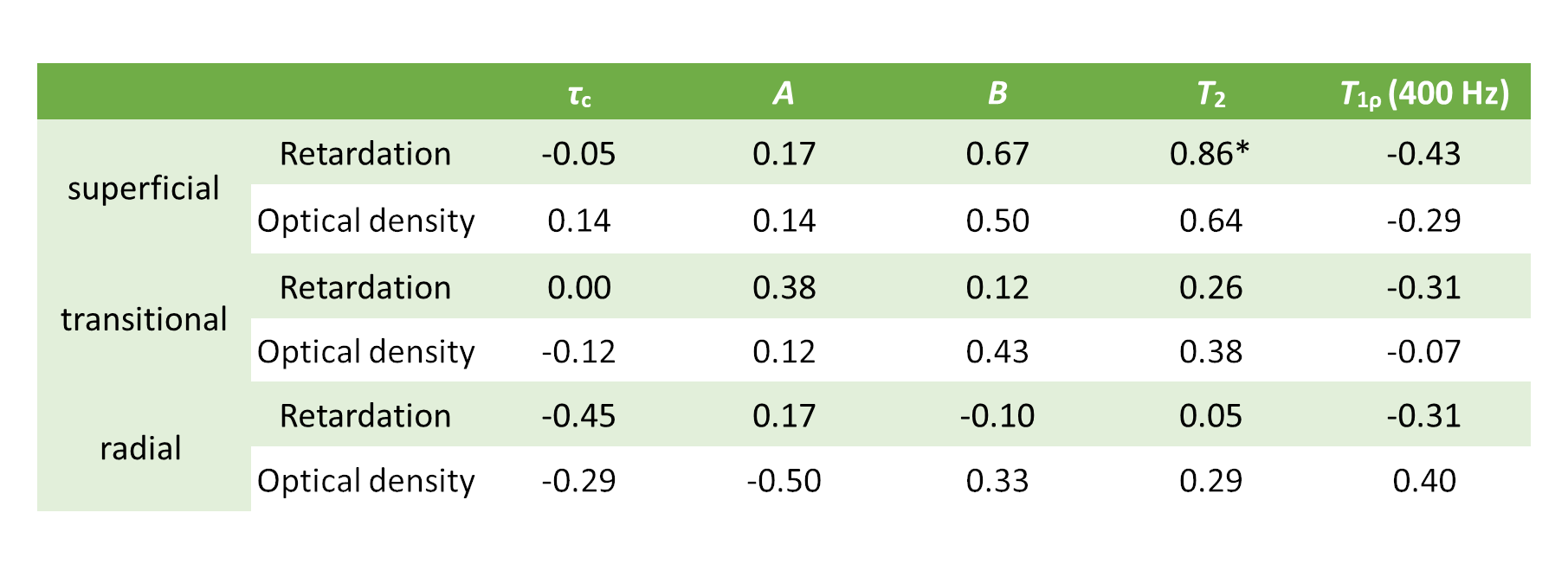
Table 2: Zonal spearman
correlation coefficients of MRI parameters: $$$\tau_c$$$, $$$A$$$, $$$B$$$,
$$$T_2$$$ and $$$T_{1\rho}$$$ at 400 Hz vs histological parameters: retardation
and optical density. The correlations are calculated from zonal mean values
pooled from all samples.