0518
Perfusion Quantification Validation on a Numerical Vascular Network of the Kidney: Traditional Kety’s Method vs Quantitative Transport Mapping
Liangdong Zhou1, Qihao Zhang1,2, Pascal Spincemaille1, Thanh D Nguyen1, John Morgan1, Weiying Dai1, Ajay Gupta1, Martin R Prince1, and Yi Wang1,2
1Weill Medical College of Cornell University, New York, NY, United States, 2Cornell University, Ithaca, NY, United States
1Weill Medical College of Cornell University, New York, NY, United States, 2Cornell University, Ithaca, NY, United States
Synopsis
Perfusion quantification is important for the diagnosis of many diseases. Validation of perfusion quantification methods remains challenging due to the various assumptions and lack of the ground truth. We built a numerical phantom of microvascular network in the kidney. In the phantom, the ground truth blood velocity and flow were computed from Navier-Stokes equation. Tracer concentration was simulated based on the mass transport equation. Comparison between Kety's method and our recently proposed AIF-free QTM method was performed using the numerical phantom. It turns out that QTM method reduces the flow error by more than 3 folds compare with Kety's method.
Introduction
Validation of tissue perfusion quantification remains challenging: the microsphere deposition approach provides arguably the best reference standard so far but is yet problematically dependent on transcapillary extraction details1-4. We propose here to validate perfusion quantification on a numerical phantom, where the true tissue perfusion quantity is known according to the law of transport physics of momentum and mass fluxes or Navier-Stokes and continuity equations5,6. Accordingly, we validate the commonly used Kety’s method for perfusion quantification, which uses an arterial input function (AIF), a global parameter that is not justifiable for all voxels in an imaging volume7-9. We also validate a novel quantitative transport mapping (QTM)10-12.Methods and Materials
$$$\hspace{1cm}{\bf\text{1.Numerical microvascular network of the kidney}}$$$The 3D shape of the kidney was obtained from the segmentation of the combination of the M0 map and ASL data. The vasculature was constructed within the segmented 3D shape of the kidney. The MRA was used to segment the renal arteries, and the directions of renal arterial branches were used to ensure that the constructed vasculature follows the correct direction pattern. Starting from the segmented renal artery branches, the microvasculature structure in the whole kidney was generated using the bifurcation branch rule13. The process of generating renal microvascular branches was stopped when the renal blood volume (RBV) in the cortex reached 16%-20%14,15. The vascular structure parameters were computed for all voxels.
We adopted the Krogh model16 to compute the blood velocity and pressure in the constructed microvascular network, and the solution of velocity was then voxelized to serve as the ground truth velocity. Given the microvascular model, the intravascular blood velocity follows the steady-state Navier-Stokes equation and the tracer concentration is governed by the continuity equation17:
$$\rho_b({\bf\,u}\cdot\nabla){\bf\,u}\,=\,-\nabla\,p+\mu\nabla\cdot\nabla{\bf\,u},\,\quad{\bf\,r}\in\Omega_v,\qquad\,(1)$$ $$\rho_b\nabla\cdot{\bf\,u}=0,\,\quad{\bf\,r}\in\Omega_v,\,\qquad(2)$$where $$$\rho_b$$$ is the density of the blood, $$$p$$$ the pressure, $$$\mu$$$ the blood viscosity, $$$\Omega_v$$$ the domain of intravascular space.
The simulated velocity and pressure were used to simulate the tracer concentration in the microvascular network using the analytical approach18,19 for:
$$\partial_tc({\bf\,r},t)=-\nabla\cdot(c({\bf\,r},t){\bf\,u}({\bf\,r}))+\nabla\cdot(D({\bf\,r})\nabla\,c({\bf r},t))-\gamma\,c({\bf\,r},t),\quad {\bf\,r}\in\Omega_v,\,(3)$$ The simulated concentration was voxelized for the use of QTM algorithm10-12 to reconstruct blood velocity and flow.
$$$\hspace{1cm}{\bf\text{2.In vivo experiment}}$$$
The QTM was tested on 7 healthy subjects with 4 post-labeling delay kidney PCASL data. Data acquisition parameters are: 3D FSE PCASL, GE MR750 3T scanner, 32 channel body coil, 2.5x2.5x4 mm3 voxel size, 128x128x36 matrix size, 10.4840ms TE, 111o flip angle, three signal averages, ~4.5 min scan time, PLD = 1025ms, 1525ms, 2025ms, 2525ms, background suppression, synchronized breathing. At the same image acquisition session, non-contrast 3D MR angiogram (MRA) IFIR data were acquired for each subject. Acquisition parameters for the MRA include: 0.625x0.625x2 mm3 voxel size, 512x512x128 matrix size, 4.0240ms TR, 2.0120ms TE, 50o flip angle, with breath gating20.
Results
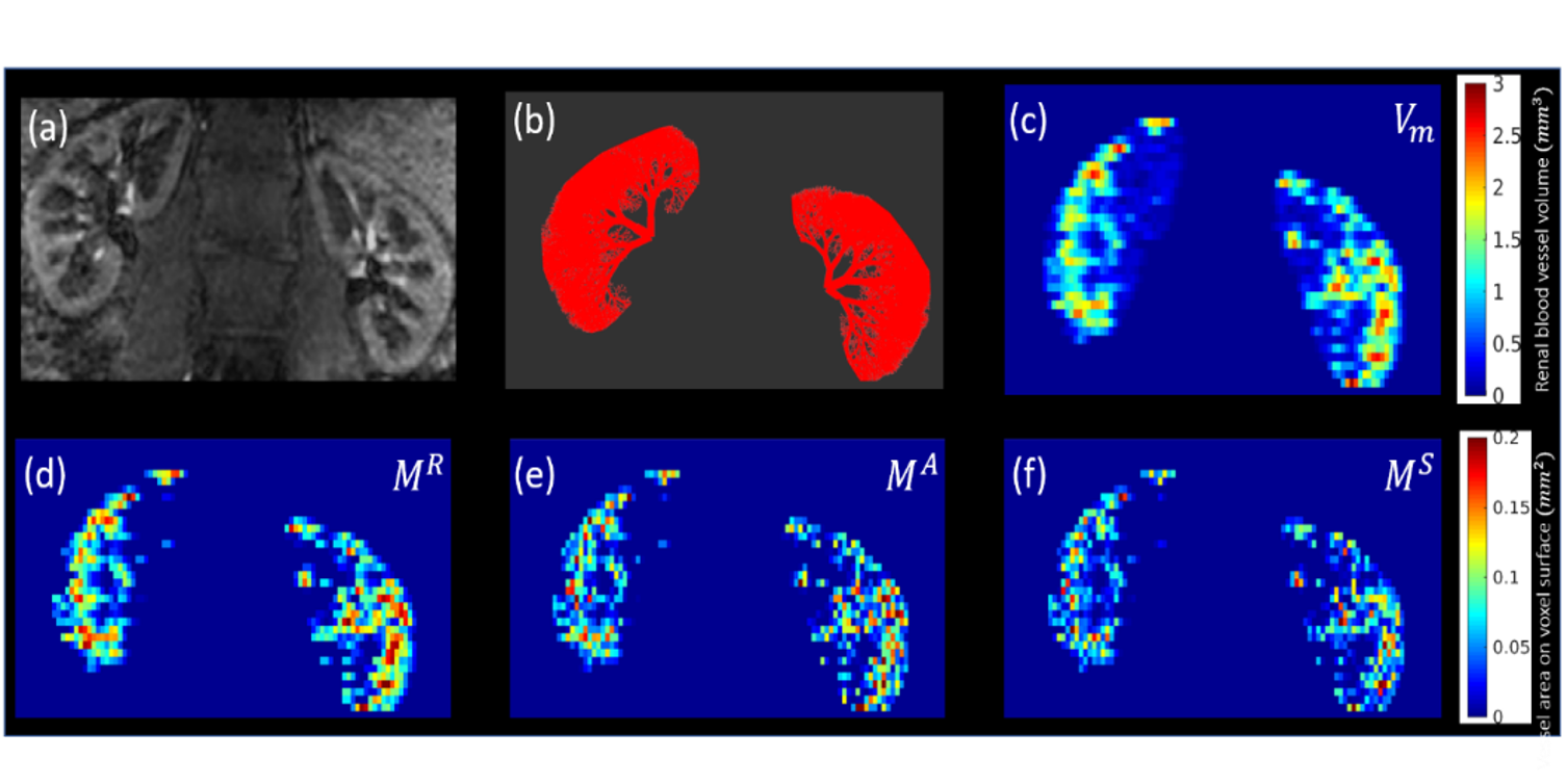
Figure 1 shows the simulated microvasculature based on the 3D kidney shape segmented from MRA and M0 data, and the corresponding structural parameters calculated from the microvascular network using voxelization.Figure 2 demonstrates the simulated forward problem solution of pressure, velocity, flow in the numerically generated microvascular network. These results were used to generate the ground truth of velocity and flow maps at the voxel level.
Figure 3 presents the simulated tracer concentration at different time points with tracer labeling duration as 1.5s. The velocity field in Figure 2 (b) was used for the tracer delivery simulation.
Figure 4 shows the comparison of numerical simulation results between ground truth, the QTM, and Kety’s method. It shows that the mean square root errors (MSRE) of estimated flow from QTM and Kety’s method are 49.7395 ml/100g/min and 169.1531 ml/100g/min, which are of 18.6% and 63.4% of the mean of the ground truth flow 266.64ml/100g/min, respectively.
Figures 5 displays the in vivo results for one healthy volunteer. QTM provides an additional velocity field map, which is not available in Kety's method. For all seven healthy subjects, the mean blood flow in the cortex was $$$498\pm46$$$ ml/100g/min and $$$556\pm36$$$ ml/100g/min for QTM and Kety’s method, respectively. For the medulla region, blood flow was $$$263\pm54$$$ ml/100g/min and $$$385\pm79$$$ ml/100g/min, for QTM and Kety’s method, respectively.
Discussion and conclusion
In the numerical phantom of kidney vasculature where the true tissue perfusion quantity is known, QTM drastically reduces Kety’s flow error by more than 3 folds. In preliminary in vivo results, automated QTM processing from multiple pulse labeling delays is feasible, but QTM generates regional blood flow different in value from Kety’s flow. It seems that Kety's method is sensitive to the error in the M0 image. The QTM model is a biophysics-based quantitative description of blood transport in the microvascular network to the tissue in which AIF is not required. Voxelization with the constructed microvasculature is needed to discretize the continuous model into voxel-level discrete space. Numerical results show that the reconstructed average blood velocity and flow maps from QTM agree well with the ground truth, yet residual error remains likely due to approximation in carrying out the very expensive computation of Eqs. 1&3. In conclusion, numerical vascular phantoms with the known ground truth of perfusion provide validation of experimental perfusion quantification methods. The novel QTM method is fairly accurate, while the traditional Kety’s method is quite erroneous.Acknowledgements
No acknowledgement found.References
- Heymann MA, Payne BD, Hoffman JI, Rudolph AM. Blood flow measurements with radionuclide-labeled particles. Prog Cardiovasc Dis 1977;20(1):55-79.
- Prinzen FW, Bassingthwaighte JB. Blood flow distributions by microsphere deposition methods. Cardiovasc Res 2000;45(1):13-21.
- Bos A, Bergmann R, Strobel K, Hofheinz F, Steinbach J, den Hoff J. Cerebral blood flow quantification in the rat: a direct comparison of arterial spin labeling MRI with radioactive microsphere PET. EJNMMI Res 2012;2(1):47.
- Artz NS, Wentland AL, Sadowski EA, Djamali A, Grist TM, Seo S, Fain SB. Comparing kidney perfusion using noncontrast arterial spin labeling MRI and microsphere methods in an interventional swine model. Invest Radiol 2011;46(2):124-131.
- Thiriet M. Biology and Mechanics of Blood Flows Part I: Biology Introduction. Biology and Mechanics of Blood Flows 2008.
- Muller A, Clarke R, Ho H. Fast blood-flow simulation for large arterial trees containing thousands of vessels. Comput Method Biomec 2017;20(2):160-170.
- Buxton RB, Frank LR, Wong EC, Siewert B, Warach S, Edelman RR. A general kinetic model for quantitative perfusion imaging with arterial spin labeling. Magnetic resonance in medicine 1998;40(3):383-396.
- Calamante F. Arterial input function in perfusion MRI: a comprehensive review. Prog Nucl Magn Reson Spectrosc 2013;74:1-32.
- Zaharchuk G. Theoretical basis of hemodynamic MR imaging techniques to measure cerebral blood volume, cerebral blood flow, and permeability. AJNR Am J Neuroradiol 2007;28(10):1850-1858.
- Spincemaille P, Zhang Q, Nguyen TD, Wang Y. Vector field perfusion imaging.Proc. Intl. Soc. Mag. Reson. Med. 25 (2017), P.3793.
- Zhou L, Spincemaille P, Zhang Q, Nguyen T, Doyeux V, Lorthois S, Wang Y. Vector Field Perfusion Imaging: A Validation Study by Using Multiphysics Model. Proc. Intl. Soc. Mag. Reson. Med. 26 (2018), P.1870.
- Zhou L, Zhang Q, Spincemaille P, Nguyen T, Wang Y. Quantitative Transport Mapping (QTM) of the Kidney using a Microvascular Network Approximation. Proc. Intl. Soc. Mag. Reson. Med. 27 (2019), P.703.
- Karch R, Neumann F, Neumann M, Schreiner W. A three-dimensional model for arterial tree representation, generated by constrained constructive optimization. Comput Biol Med 1999;29(1):19-38.
- Yamashita M, Inaba T, Oda Y, Mizukawa N. Renal blood volume vs. glomerular filtration rate: evaluation with C15O and 88Ga-ethylenediaminetetraacetic acid (EDTA) study. Radioisotopes 1989;38(9):373-376.
- Kudomi N, Koivuviita N, Liukko KE, Oikonen VJ, Tolvanen T, Iida H, Tertti R, Metsarinne K, Iozzo P, Nuutila P. Parametric renal blood flow imaging using [O-15]H2O and PET. Eur J Nucl Med Mol I 2009;36(4):683-691.
- Lorthois S, Cassot F, Lauwers F. Simulation study of brain blood flow regulation by intra-cortical arterioles in an anatomically accurate large human vascular network: Part I: methodology and baseline flow. Neuroimage 2011;54(2):1031-1042.
- Secomb TW. Hemodynamics. Compr Physiol 2016;6(2):975-1003.
- Chen JS, T. CJ, W. LC, P. LC, W LC. Analytical solutions to two-dimensional advection–dispersion equation in cylindrical coordinates in finite domain subject to first- and third-type inlet boundary conditions. Journal of Hydrology 2011;405:10.
- Massabo M, Cianci R, Paladino O. Some analytical solutions for two-dimensional convection-dispersion equation in cylindrical geometry. Environ Modell Softw 2006;21(5):681-688.
- Rajendran R, Lew SK, Yong CX, Tan J, Wang DJJ, Chuang KH. Quantitative mouse renal perfusion using arterial spin labeling. NMR in biomedicine 2013;26(10):1225-1232.
Figures
Figure
1: Illustration of microvasculature construction and structural parameters. (a)
Renal MRA image with arteria information shown with the bright signal; (b) constructed microvasculature in the kidney using the renal
arterial vessel information and shape information from MRA image in (a); (c)
calculated renal
blood vessel absolute volume map (unit: $$$mm^3)$$$ from constructed microvasculature in (b); (d)-(f) calculated intersectional
areas $$$M^R,M^A,M^S$$$ (unit: $$$mm^2$$$)
of blood vessel on the Right, Anterior, and Superior surfaces of a voxel,
respectively.
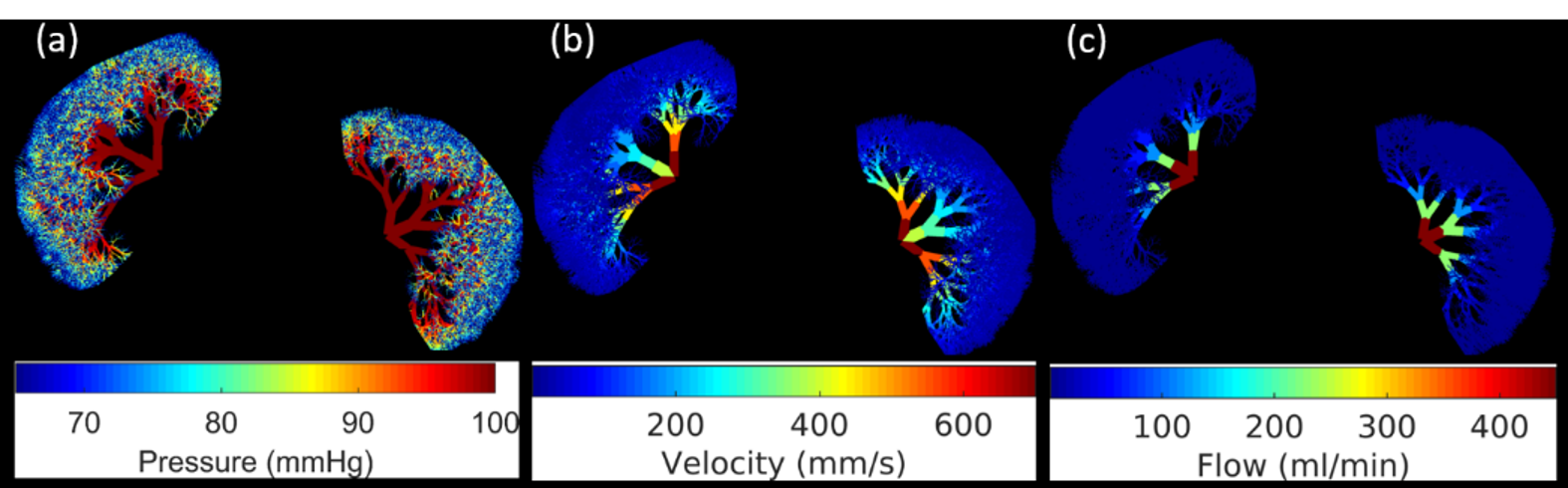
Figure 2: Numerical simulation results of the forward problem in the microvascular network in the kidney: (a) blood pressure distribution (mmHg), (b) blood velocity distribution (mm/s), (c) blood flow rate (ml/min). These solutions need to be voxelized to the image voxel level to serve as the ground truth of the QTM inverse problem.
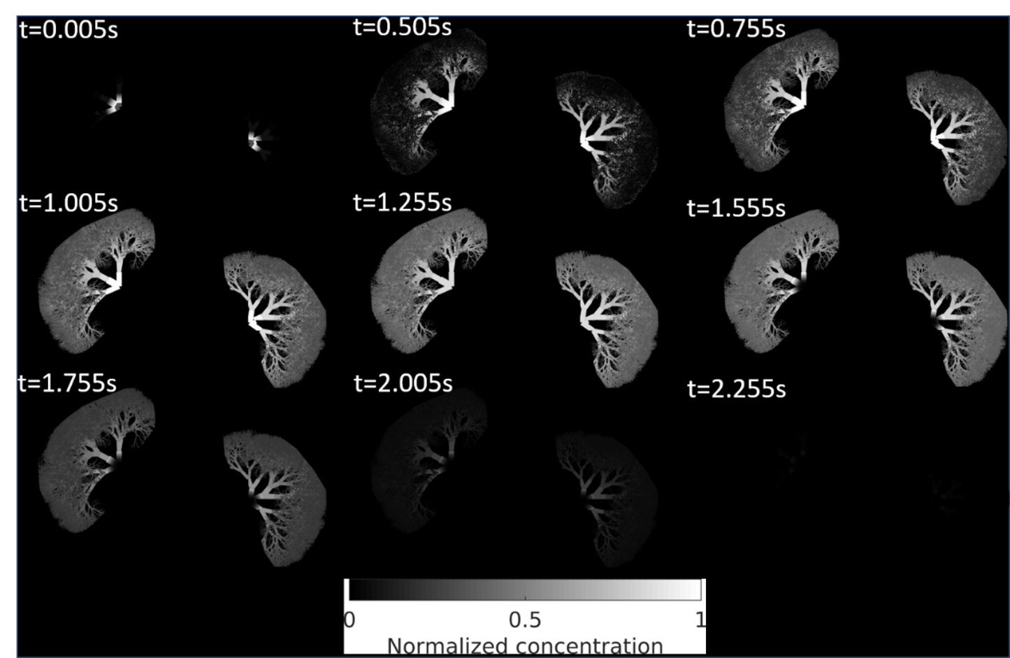
Figure 3: Simulated solution of tracer concentration at 9 time frames in the simulated microvascular network of a kidney using the velocity in Fig.2(b). These tracer concentrations need to be voxelized to the image voxel level to serve as the input of the QTM inverse problem.
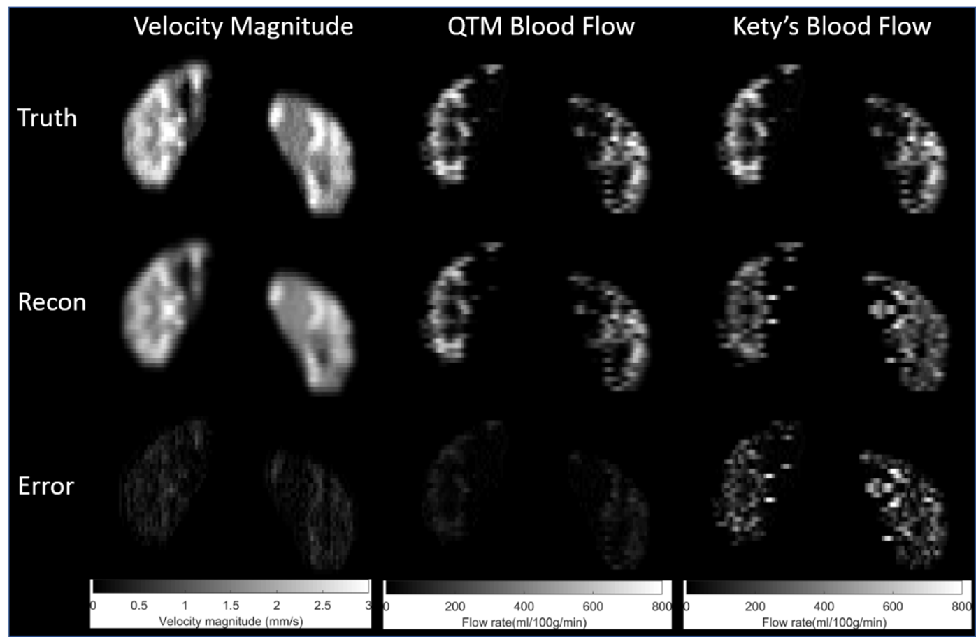
Figure
4: The numerical results comparison between QTM, Kety’s
method, and the ground truth. The first, second, and third columns are velocity
magnitude, QTM blood flow, and Kety’s
blood flow, respectively. The first, second, and third rows are ground truth,
reconstruction, and the absolute error between reconstruction and the ground
truth. respectively. The RMSE of flow for QTM and Kety's method are 49.7395
ml/100g/min and 169.1531 ml/100g/min, which are of 18.6% and 63.4% of the mean
of the ground truth flow 266.64ml/100g/min, respectively.
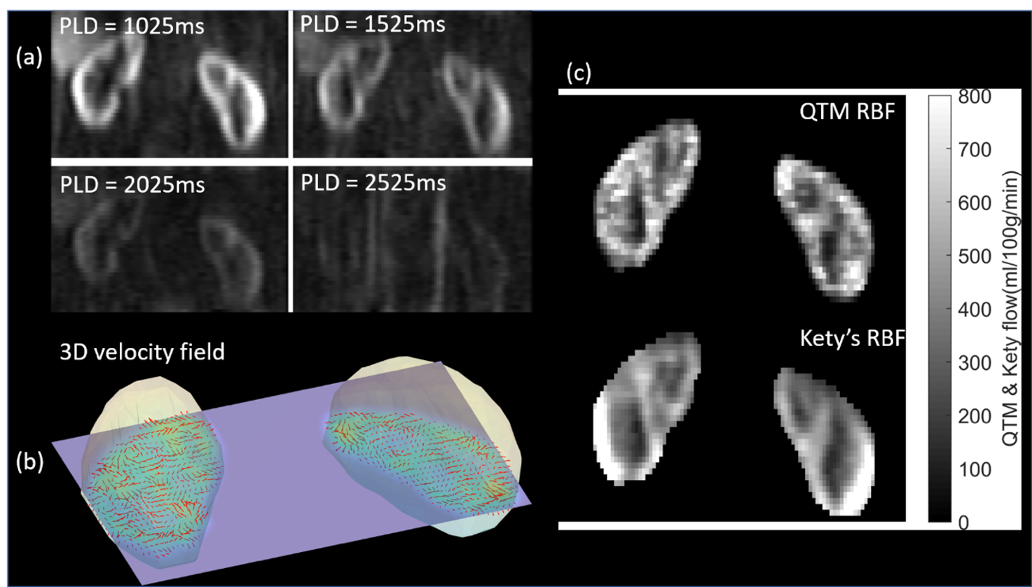
Figure 5: QTM results of a healthy volunteer. (a) the ASL data at four
PLDs = 1s, 1.5s, 2s, 2.5s (left to right, top to bottom); (b) the 3D display of
the vector field from QTM on one slice; (c) the renal blood flow comparison
between QTM (top) and
Kety’s method (bottom). It shows that results from QTM were more realistic than those from Kety's method since RBF in Kety's results was not homogeneous in the renal cortex region due to the error in M0 images. It turns out that Kety's method is more sensitive to the artifacts in M0 images and the parameters including blood arrival time, labeling efficiency.