0509
DeepCEST 3T: Robust neural network prediction of 3T CEST MRI parameters including uncertainty quantification1Magnetic Resonance Center, Max Planck Institute for Biological Cybernetics, Tübingen, Germany, 2Department of Perceiving Systems, Max Planck Institute for Intelligent Systems, Tübingen, Germany, 3Department of Diagnostic and Interventional Neuroradiology, Eberhard Karls University Tübingen, Tübingen, Germany, 4Department of Biomedical Magnetic Resonance, Eberhard Karls University Tübingen, Tübingen, Germany, 5Department of Neuroradiology, University Clinic Erlangen, Erlangen, Germany
Synopsis
Analysis of CEST data often requires complex mathematical modeling before contrast generation, which can be error prone and time-consuming. Here, a probabilistic deep learning approach is introduced to shortcut conventional Lorentzian fitting analysis of 3T in-vivo CEST data by learning from previously evaluated data. It is demonstrated that the trained networks generalize to data of a healthy subject and a brain tumor patient, providing CEST contrasts in a fraction of the conventional evaluation time. Additionally, the probabilistic network architecture enables uncertainty quantification, indicating if predictions are trustworthy, which is assessed by perturbation analysis.
Introduction
Calculation of sophisticated MR contrasts often requires complex mathematical modeling, which can be computationally expensive and sensitive to fit algorithm parameters. In this work, we investigate whether neural networks (NNs) can provide not only a shortcut to conventional fitting, but also a quality metric for the predicted values, so-called uncertainty quantification, investigated here in the context of multi-pool Lorentzian fitting of CEST-spectra at 3T. The uncertainties allow radiographers to interpret the generated CEST maps with high confidence.Methods
Z-spectra at 55 frequency offsets between ±100ppm were acquired from 4 healthy subjects and one brain tumor patient at 3 different sites with identical 3T whole-body MRI systems (MAGNETOM Prisma, Siemens Healthcare, Erlangen, Germany) after written informed consent, using a 3D snapshot-CEST sequence1 and a low-power pre-saturation block2.Z-spectra were de-noised by principal component analysis using the median truncation criterion3. A four-pool Lorentzian fit model4 was used describing direct water saturation (DS), semi-solid magnetization transfer (MT), amide (APT) and relayed NOE peaks. The model includes the water frequency shift δDS as free parameter and thus takes B0 inhomogeneity into account.
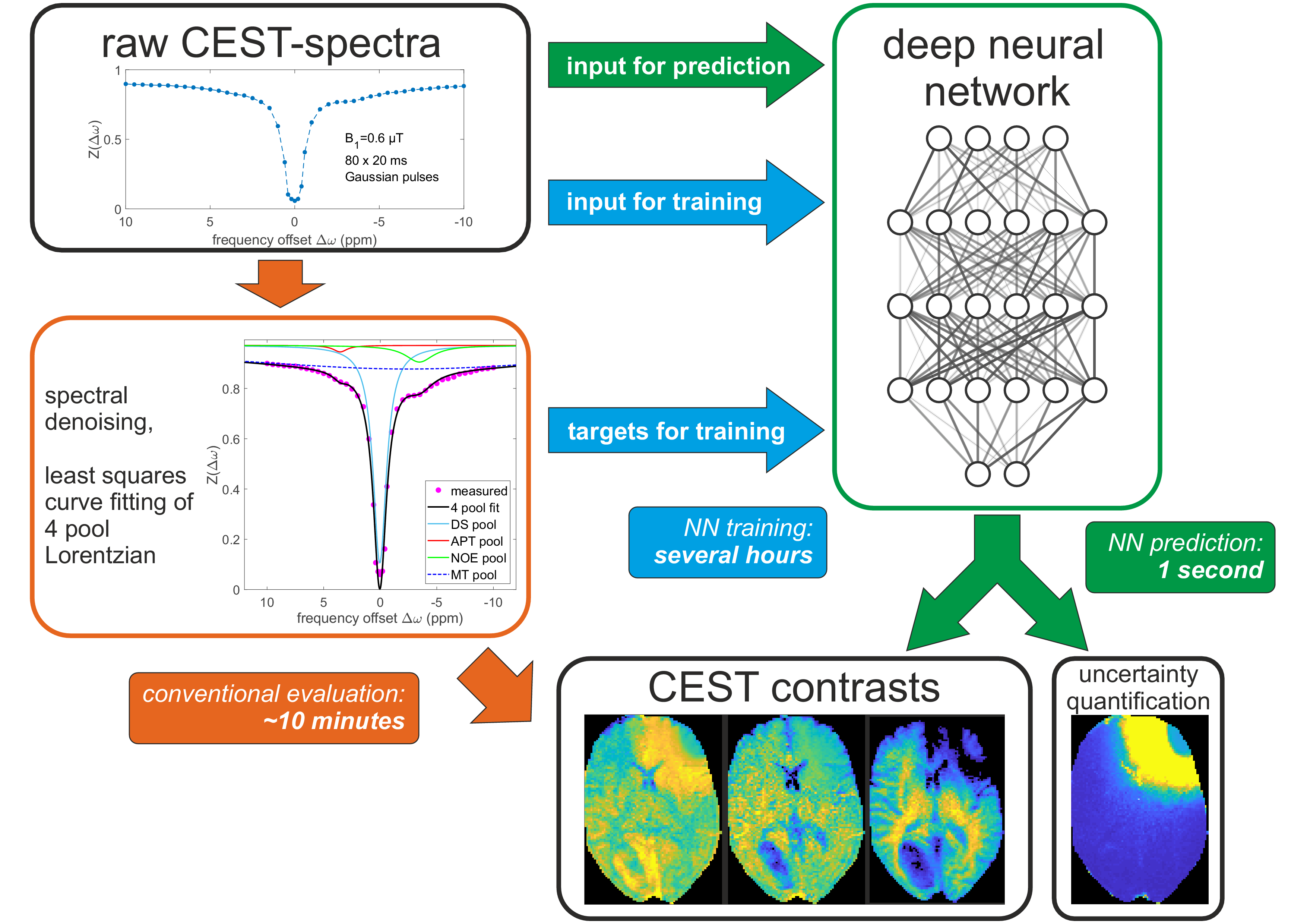
Deep feed-forward NNs were set up in tensorflow5/keras6 to map vectors $$$x$$$ of 55 elements representing raw Z-spectra to vectors $$$\mu(x)=(\mu_1(x),...,\mu_n(x))$$$ of $$$n=10$$$ elements, representing the free parameters of the Lorentzian model. Following approaches of learned output variance via maximum-likelihood estimation employed in computer vision7–9, the NN has 10 additional output neurons representing uncertainties $$$\sigma(x)=(\sigma_1(x),...,\sigma_n(x))$$$ of each Lorentzian parameter. These uncertainty outputs are indirectly inferred from the training data by training with a Gaussian negative log-likelihood loss function $$-\log p_\theta(\mu^{\text{tgt}},\mu(x),\sigma(x))=\frac{1}{2} \sum_{i=1}^{n}\left(\frac{\mu^{\text{tgt}}_i-\mu_i(x)}{\sigma_i(x)}\right)^2+\sum_{i=1}^{n}\log(\sigma_i(x))+\frac{n}{2}\log(2\pi)$$ with the ground-truth training targets $$$\mu^{\text{tgt}}_{i}$$$ obtained by conventional least squares fitting. The workflow is shown in Figure 1.
A network called NN1 was trained on the combined datasets of 3 healthy subjects and tested on the fourth healthy subject and tumor patient datasets. Training data augmentation with simulated Gaussian noise in the inputs and with additional simulated B0 shifts in a range of ±0.8 ppm was employed. Overfitting was avoided by early stopping with 10 % of the data used as validation set. NN hyperparameters were optimized by a grid search, resulting in 2 layers with 100 neurons each and ELU activation.
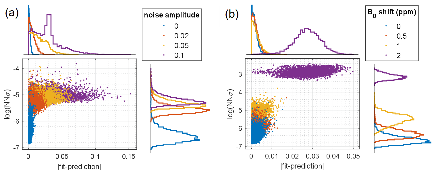
Uncertainty quantification was assessed by input perturbations with Gaussian noise and additional B0 shifts of various strengths. Additionally, an implant-like B0-artifact caused by a magnetic dipole in the tumor patient’s skull was simulated.
Results
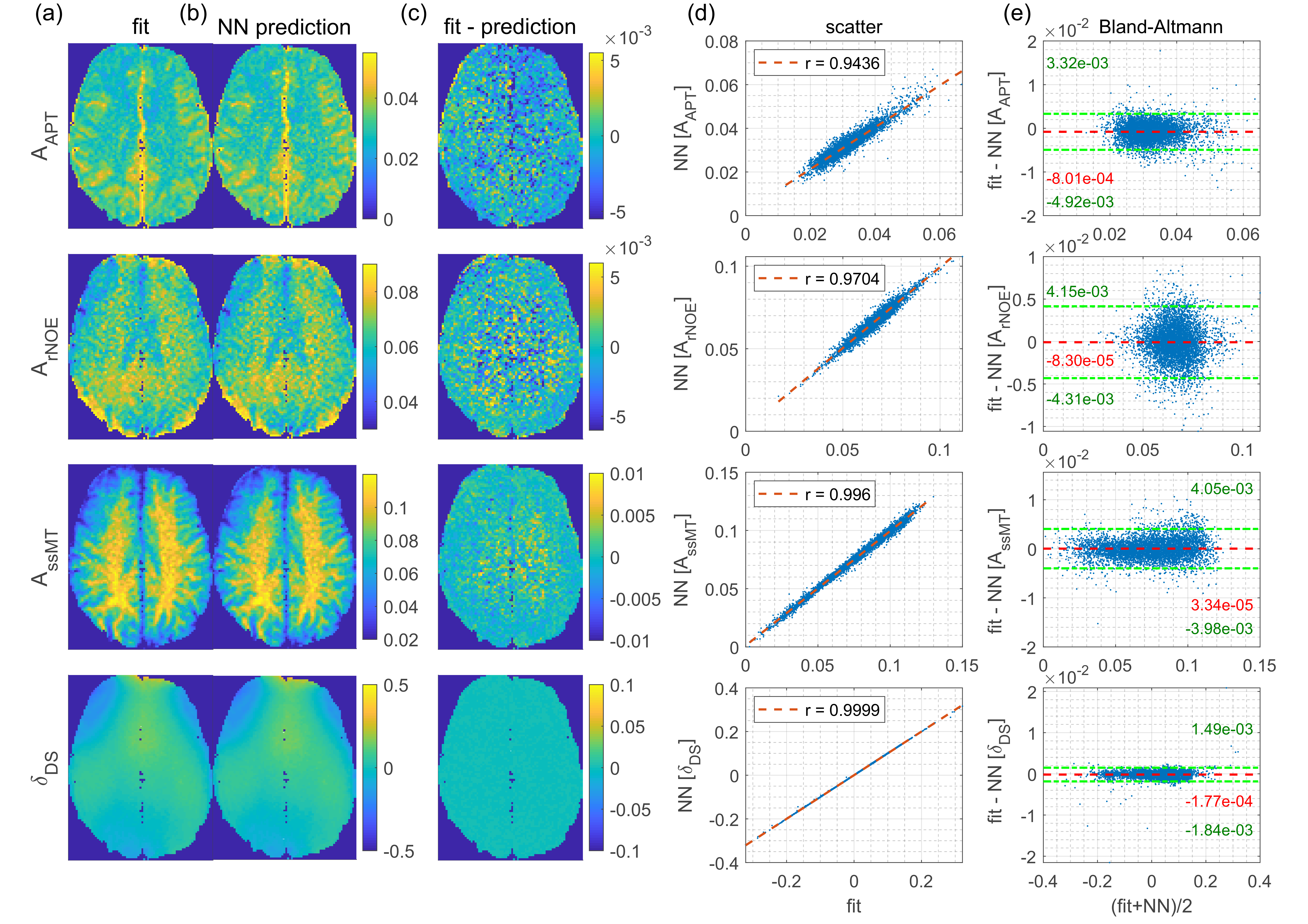
NN1 generalizes to the unseen healthy subject test dataset, as the predicted parameter maps (Figure 2b) closely match the ground truth Lorentzian fit results (Figure 2a), resulting in low prediction errors (Figure 2d). This is confirmed by scatter (Figure 2d) and Bland-Altmann analysis (Figure 2e).For input perturbation with noise (Figure 3a), strongly increased uncertainty outputs for all corrupted voxels reflect the larger prediction errors caused by fluctuations in the inputs. For perturbation with simulated B0 shifts ≥1 ppm (Figure 3b), uncertainties are significantly increased, as these shifts exceed the range covered by the training data. Thus, the uncertainty quantification recognizes corrupted and “out-of-training-data” inputs.
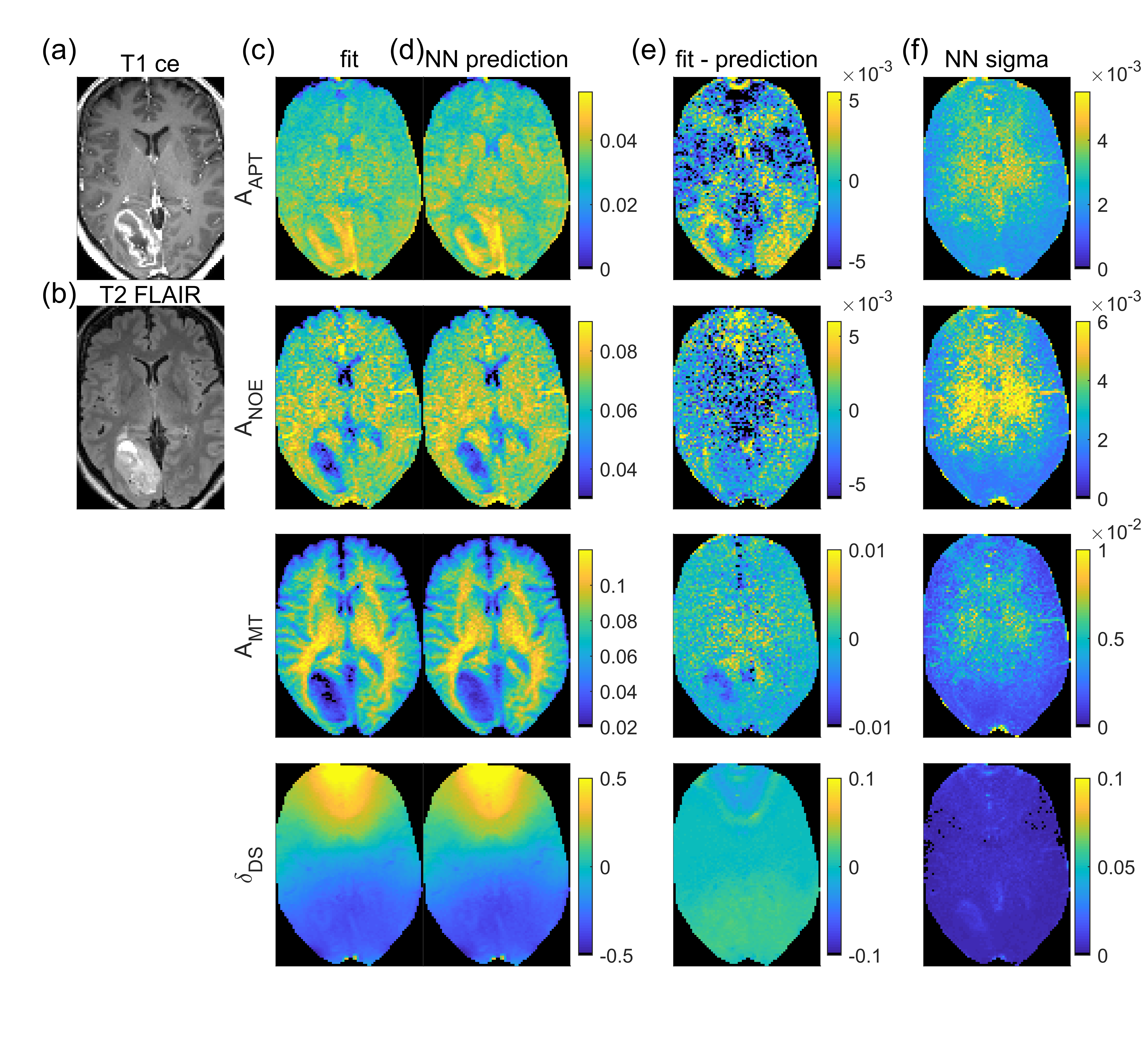
NN1 predictions from the tumor patient dataset (Figure 4d) show similar contrasts as the fit (Figure 4c), with APT hyperintensity in the tumor area. Pearson correlation coefficient r between ground truth and prediction is larger than 0.87 for all parameters. The uncertainty maps given in Figure 4e show increased values in the center of the displayed slice where SNR is lower, in parts of the tumor area – especially in the T2-FLAIR hyperintense region (Figure 4b) – and in vessels, which can show noise-like pulsation artifacts.
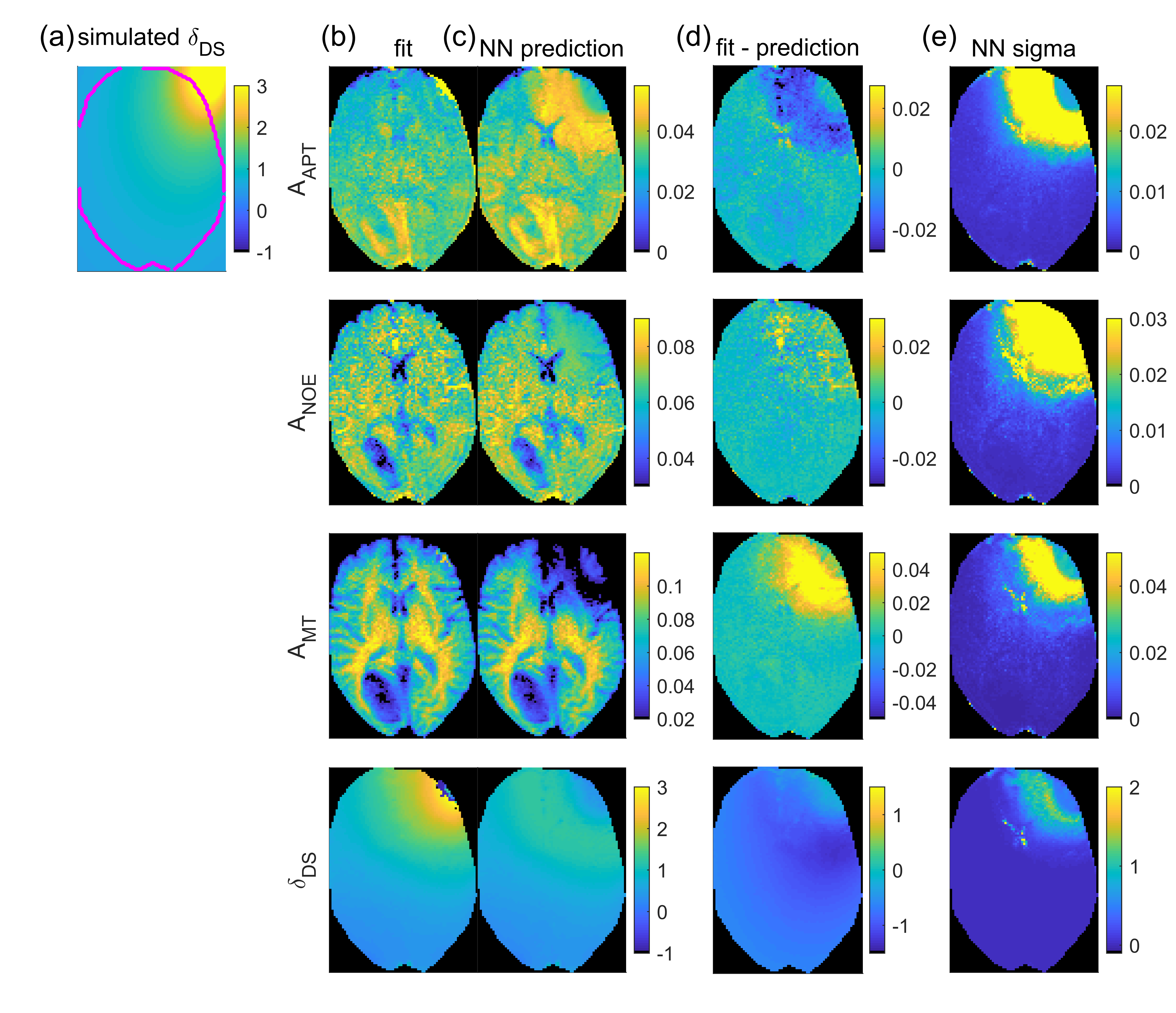
For the simulated implant-like B0-artifact, strongly increased uncertainties (Figure 5e) indicate failure of the prediction (Figure 5d) close to the dipole location, where the strong field inhomogeneity (Figure 5a) shifts Z-spectra drastically. Thus, contrast that might arise from or is depleted by the B0 artifact can be identified by means of the uncertainty maps and therefore not be misinterpreted.
Discussion
The trained NN generates CEST contrasts from uncorrected Z-spectra rapidly (~1s for ~50,000 Z-spectra as opposed to ~10min in case of Lorentzian fitting) and accurately, generalizing to data that was not included in training. A limitation is introduced by the fact that training data itself is generated by least squares Lorentzian fitting. This is a simplified model and suffers from typical instabilities caused by low SNR and dependence on initial and boundary values. Thus, the current approach proves the concept of a shortcut to conventional fitting including uncertainty quantification but can be extended to improved Z-spectrum models such as Bloch-McConnell fitting10–12.Using NNs as shortcut for least squares fitting has been proposed before13, also in the context of MRI14–16 and CEST17–19. However, none of these approaches includes uncertainty quantification. The presented probabilistic output layer can be easily adapted to other regression NNs, enabling uncertainty quantification for similar approaches.
Conclusion
The deepCEST NN allows fast estimation of CEST parameters, providing a shortcut to the conventional evaluation method at 3T. Moreover, the introduced uncertainty quantification indicates if the predictions are trustworthy, enabling confident interpretation of contrast changes. This is promising for fast online reconstruction, bringing sophisticated CEST contrasts a step closer to clinical application.Acknowledgements
Max Planck Society; German Research Foundation (DFG, grant ZA 814/2-1, support to KH); European Union Horizon 2020 research and innovation programme (Grant Agreement No. 667510, support to MZ, AD).References
1. Zaiss M, Ehses P, Scheffler K. Snapshot-CEST: Optimizing spiral-centric-reordered gradient echo acquisition for fast and robust 3D CEST MRI at 9.4 T. NMR in Biomedicine. 2018;31(4):e3879. doi:10.1002/nbm.3879
2. Deshmane A, Zaiss M, Lindig T, et al. 3D gradient echo snapshot CEST MRI with low power saturation for human studies at 3T. Magnetic Resonance in Medicine. 2019;81(4):2412-2423. doi:10.1002/mrm.27569
3. Breitling J, Deshmane A, Goerke S, et al. Adaptive denoising for chemical exchange saturation transfer MR imaging. NMR in Biomedicine. 2019;0(0):e4133. doi:10.1002/nbm.4133
4. Goerke S, Soehngen Y, Deshmane A, et al. Relaxation-compensated APT and rNOE CEST-MRI of human brain tumors at 3 T. Magnetic Resonance in Medicine. March 2019. doi:10.1002/mrm.27751
5. Abadi M, Barham P, Chen J, et al. TensorFlow: A System for Large-Scale Machine Learning. In: 12th USENIX Symposium on Operating Systems Design and Implementation (OSDI ’16). ; 2016:265-283. https://www.usenix.org/conference/osdi16/technical-sessions/presentation/abadi. Accessed June 4, 2019.
6. Chollet F, others. Keras. https://github.com/fchollet/keras. Published 2015. Accessed January 7, 2019.
7. Kendall A, Gal Y. What Uncertainties Do We Need in Bayesian Deep Learning for Computer Vision? In: Guyon I, Luxburg UV, Bengio S, et al., eds. Advances in Neural Information Processing Systems 30. Curran Associates, Inc.; 2017:5574–5584.
8. Prokudin S, Gehler P, Nowozin S. Deep Directional Statistics: Pose Estimation with Uncertainty Quantification. In: Ferrari V, Hebert M, Sminchisescu C, Weiss Y, eds. Computer Vision – ECCV 2018. Vol 11213. Cham: Springer International Publishing; 2018:542-559. doi:10.1007/978-3-030-01240-3_33
9. Gast J, Roth S. Lightweight Probabilistic Deep Networks. In: 2018 IEEE/CVF Conference on Computer Vision and Pattern Recognition; 2018:3369-3378.
10. Heo H-Y, Zhang Y, Lee D-H, Hong X, Zhou J. Quantitative assessment of amide proton transfer (APT) and nuclear overhauser enhancement (NOE) imaging with extrapolated semi‐solid magnetization transfer reference (EMR) signals: Application to a rat glioma model at 4.7 tesla. Magnetic Resonance in Medicine. 2016;75(1):137-149. doi:10.1002/mrm.25581
11. Heo H-Y, Zhang Y, Jiang S, Lee D-H, Zhou J. Quantitative assessment of amide proton transfer (APT) and nuclear overhauser enhancement (NOE) imaging with extrapolated semisolid magnetization transfer reference (EMR) signals: II. Comparison of three EMR models and application to human brain glioma at 3 Tesla. Magnetic Resonance in Medicine. 2016;75(4):1630-1639. doi:10.1002/mrm.25795
12. Liu D, Zhou J, Xue R, Zuo Z, An J, Wang DJJ. Quantitative characterization of nuclear overhauser enhancement and amide proton transfer effects in the human brain at 7 Tesla. Magnetic Resonance in Medicine. 2013;70(4):1070-1081. doi:10.1002/mrm.24560
13. Bishop CM, Roach CM. Fast curve fitting using neural networks. Review of Scientific Instruments. 1992;63(10):4450-4456. doi:10.1063/1.1143696
14. Bertleff M, Domsch S, Weingärtner S, et al. Diffusion parameter mapping with the combined intravoxel incoherent motion and kurtosis model using artificial neural networks at 3 T. NMR in Biomedicine. 2017;30(12):e3833. doi:10.1002/nbm.3833
15. Domsch S, Mürle B, Weingärtner S, Zapp J, Wenz F, Schad LR. Oxygen extraction fraction mapping at 3 Tesla using an artificial neural network: A feasibility study. Magnetic Resonance in Medicine. 2018;79(2):890-899. doi:10.1002/mrm.26749
16. Liu H, Xiang Q-S, Tam R, MacKay A, Kramer J, Laule C. 150× acceleration of myelin water imaging data analysis by a neural network, Program Number 0152. In: Proceedings of ISMRM 27th Annual Meeting; 2019.
17. Chen L, Schär M, Chan KWY, et al. High-resolution phosphocreatine mapping of human skeletal muscle by artificial neural network-based chemical exchange saturation transfer MRI at 3T, Program Number 0048. In: Proceedings of ISMRM 27th Annual Meeting; 2019.
18. Deshmane A, Zaiss M, Herz K, Bender B, Lindig T, Scheffler K. Machine Learning accelerates and stabilizes selective CEST fitting at 3T, Program Number 5002. In: Proceedings of ISMRM 27th Annual Meeting; 2019.
19. Glang F, Deshmane A, Martin F, Herz K, Scheffler K, Zaiss M. Can a neural network predict B0 maps from uncorrected CEST-spectra? Program Number 4995. In: Proceedings of ISMRM 27th Annual Meeting; 2019.
Figures