Introduction

MRI scanning is sensitive to subject motion due to lengthy data acquisition, which is longer than most types of physiological movement cycles [1]. In order to reduce scanning time and the impact from motion, parallel imaging methods have been introduced and applied in clinical applications. Among these methods, the recently introduced wave-CAIPI [2] achieves significantly lower g-factor penalty to image signal-to-noise ratio (SNR) than the traditional SENSE and GRAPPA methods. Thus, it is capable to achieve a high acceleration factor and reduce the scan time of the whole-brain anatomical scan with a sub-millimeter resolution from ~5 to less than 1 minute [3]. Even though the scan time has been significantly shortened, significant motion-related image degradation using wave-CAIPI acquisition can persist, for example, due to short sudden movement, in particular in the readout direction. This study proposes and investigates the possibility of using joint optimization to estimate and correct motion for accelerated 3D wave-CAIPI acquisition.

Methods

Data were acquired on a 3T MRI scanner (Prisma, Siemens AG, Erlangen, Germany) with a 32-channel head coil. A grapefruit was used as phantom, with the possibility of moving it from the outside of the magnet bore. The motion of the phantom was limited to translational movement within ±5 mm.
Data acquisition: The GRE sequence with wave-encoding and butterfly navigator [4] features was in-house developed using IDEA. The common parameters for all scans were: TR 17ms, TE 8.5 ms, flip angle 20 degrees, matrix size 192×192×96 with 1 mm isotropic voxel size. For all the wave-CAIPI sequence, a sin and a cos wave were applied on Y and Z gradient axis, respectively, during the readout window with 7 cycles and 6 mT/m in amplitude. The following sequences were implemented in this study: (1) Full sampled Cartesian GRE without motion, scan time 5 min 15 s; (2) Accelerated wave-encoded GRE (Ry = 2, Rz = 4, kz blip = 2) without motion, scan time ~ 40 s; (3) Accelerated wave-CAIPI GRE (Ry = 2, Rz = 4, kz blip = 2) with motion, scan time ~ 40s. Butterfly navigators were acquired for sequence 3.
Data processing: Image reconstruction and motion estimation/correction were performed in MATLAB (R2018b, MathWorks, MA, USA). Coil sensitivity map was calculated with Berkeley Advanced Reconstruction Toolbox (BART) through ESPIRiT [5], and the SENSE-type reconstruction was used for the wave-CAIPI datasets.
The forward model $$$E$$$ that transforms image to each k-space line with consideration of rigid-body motion $$$\phi$$$ and wave-encoding phase $$$P$$$ is:
$$s=Ex=UF_{p}CT_{\phi}R_{\phi}x$$
where $$$x$$$ is the original object, $$$s$$$ is the acquired k-space data, $$$U$$$ is the k-space location mask, $$$F$$$ is Fourier transform operator with extra wave-encoding phase $$$P$$$ along the readout direction, $$$C$$$ is coil sensitivity map, $$$T$$$ and $$$R$$$ are translation and rotation operators due to motion trajectory $$$\phi$$$. The initial values of motion were determined by the butterfly navigator instead of random assigning for faster convergence in optimization.
Joint optimization with the following target function was used to the selected target voxels for simultaneously estimating the image $$$x$$$, wave-encoding phase $$$P$$$, and motion trajectory $$$\phi$$$:
$$argmin_{x,P,\phi}||s-Ex||_{2}^{2}$$
The point spread image of a single voxel was simulated, given the same under-sampling pattern, theoretical wave-encoding as sequence 3, and the motion initial values. This point spread image was used for selecting the pattern of target voxels in 3D image domain, and this selected pattern was moved in each iteration during optimization to cover the whole spatial area, similar as in ref [6].

Results and Discussion

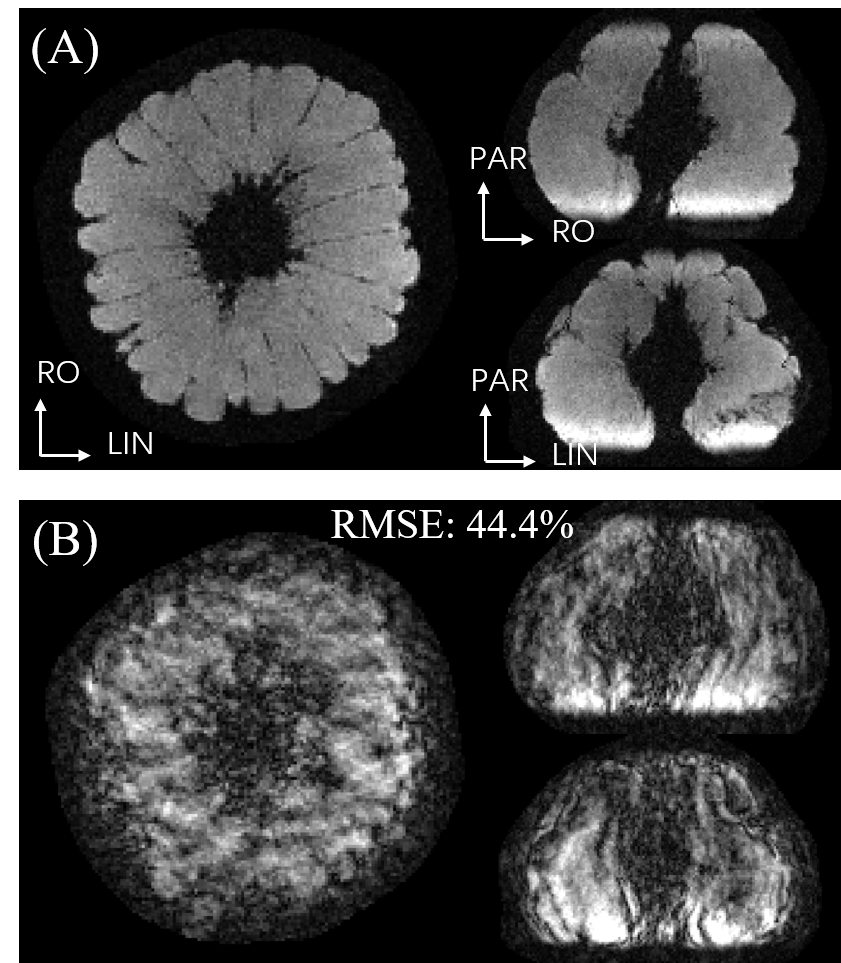
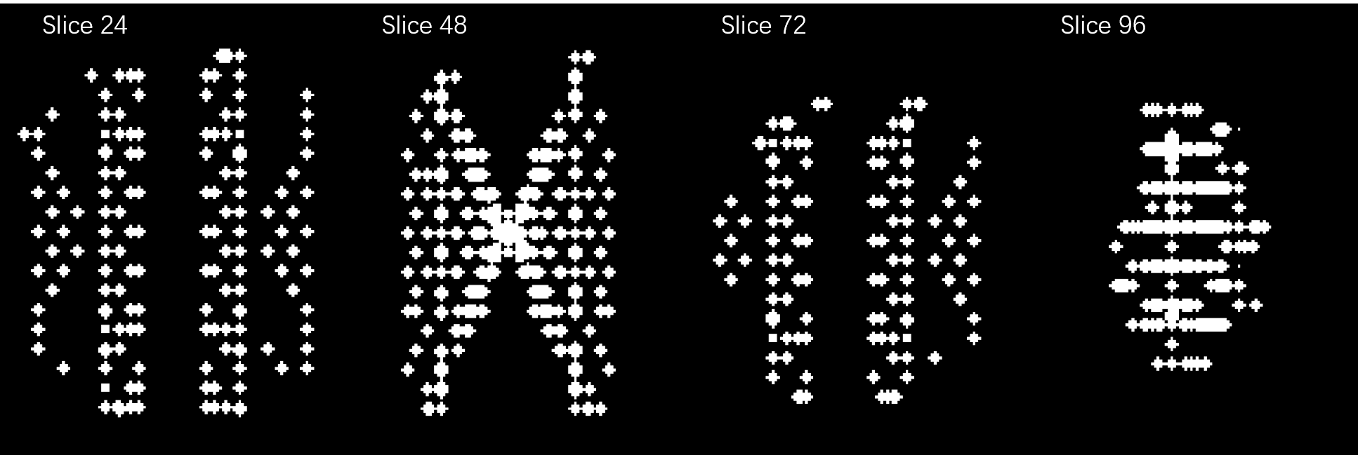
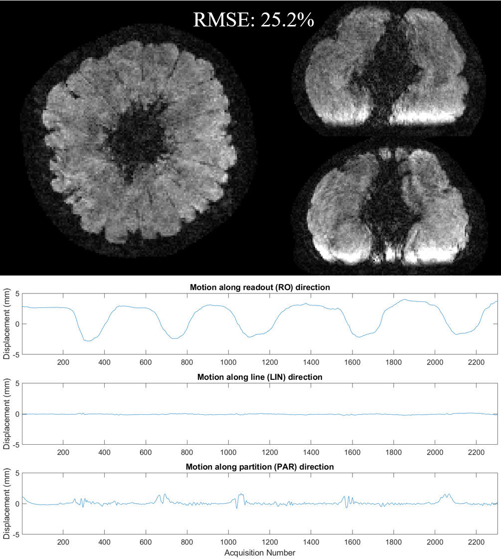
Figure 1 shows the comparison of the direct reconstruction results between no motion and motion-impacted wave-CAIPI 8× accelerated dataset. Unlike Cartesian images, motion artifact of wave-CAIPI images are not only along phase encoding directions, but also along readout direction. Figure 2 shows the point spread pattern under the scanning condition of sequence 3 on four slices. The point spread pattern is only along PE directions in Cartesian case. In contrast, in wave-CAIPI case, this point spread pattern is also along readout direction with a larger coverage, allowing smaller times of pattern shifting to cover the whole 3D FOV. Figure 3 shows the motion corrected wave-CAIPI images and the estimated motion trajectory. While mild level of motion artifacts still remain, image quality was dramatically improved, making the images comparable to the “no motion” ones. The root-mean-squared error to the non-motion wave-CAIPI scan reduced from 44.4% to 25.2%

Conclusion

Parallel imaging using wave-CAIPI significantly reduced scanning time with low g-factor penalty to image SNR. However, it is still sensitive to within-scan motion and the motion artifacts are along all three spatial dimensions. This study revealed that the motion in wave-CAIPI images could be estimated and mitigated through joint optimization on targeted voxels selected by the simulation of point spread pattern. Accuracy and algorithm performance are currently optimized in an ongoing study.

Acknowledgements

KU received funding from IBS (#IBS-R015-D1). The authors appreciate the support from Dr. Morgan Barense, Dr. Ali Golestani and Ms. Priya Abraham from Toronto Neuroimaging Facility (ToNI), Department of Psychology, University of Toronto.