0396
Processing of muscle phosphorus 7T CSI data using PCA denoising and deconvolution1Department of Radiology, UMC Utrecht, Utrecht, Netherlands
Synopsis
Chemical shift imaging generally suffers from low SNR and low spatial resolution, especially for x-nuclei. State of the art image processing methods from the MRI domain, e.g. DTI pre-processing, can be applied to CSI data. In this study we show the feasibility of PCA denoising combined with deconvolution to enhance CSI SNR and spatial localization.
Introduction
Chemical shift imaging generally suffers from low SNR and low spatial resolution, especially for X-nuclei (1). However, with current advances in transmit and receive coils, 3D CSI data sets covering larger FOV’s and with increased number of voxels are becoming available. As such, the data is becoming more suited for state-of-the-art image processing tools developed for the MRI domain, e.g. DTI pre-processing methods. In this study, we show the feasibility of PCA denoising combined with deconvolution to enhance CSI SNR and spatial localization. The proposed processing methods are shown on simulated and phantom data and are tested on in vivo upper leg 3D 31P CSI data acquired using a volume transmit coil and an array of local receivers.Methods
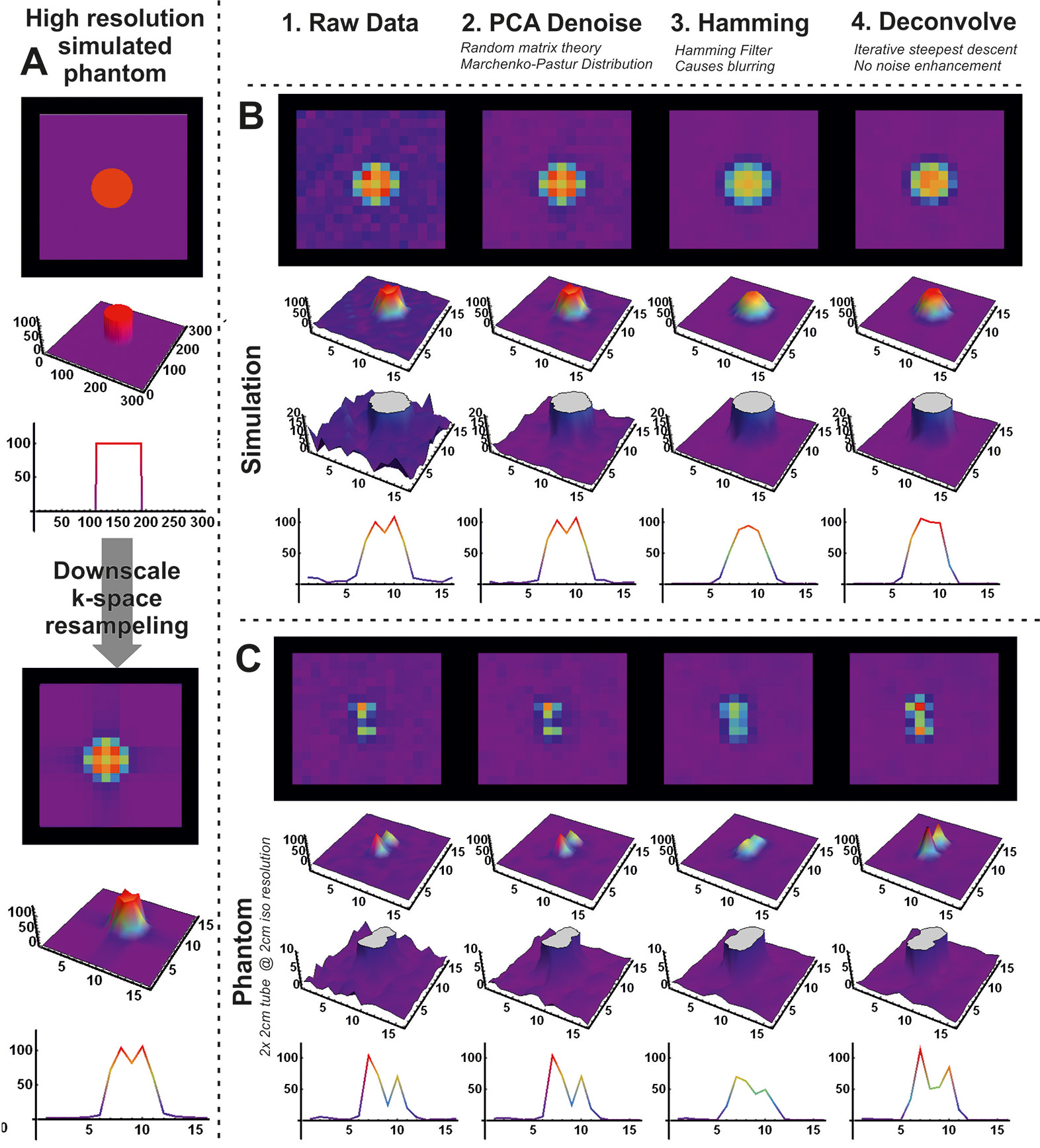
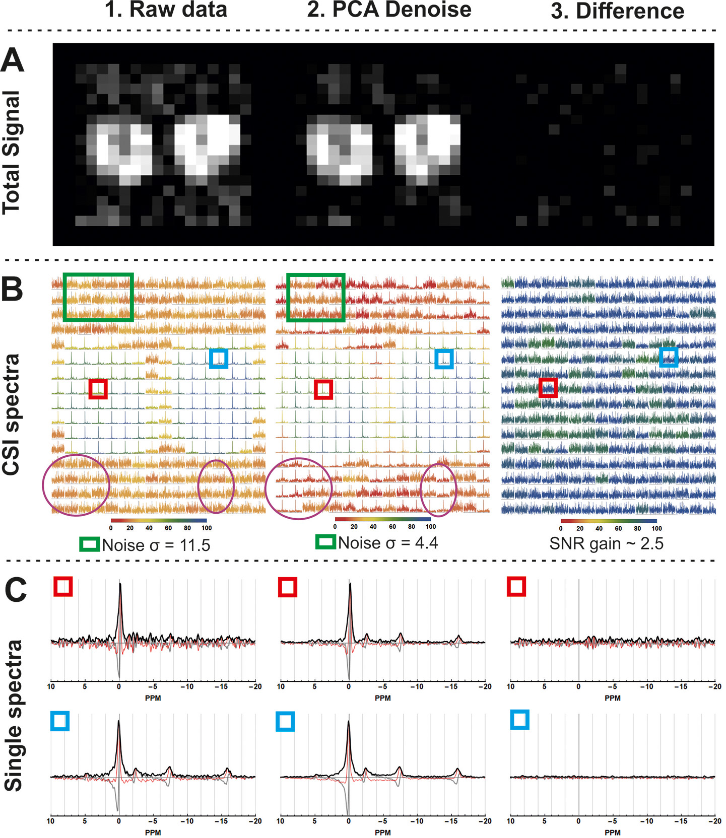
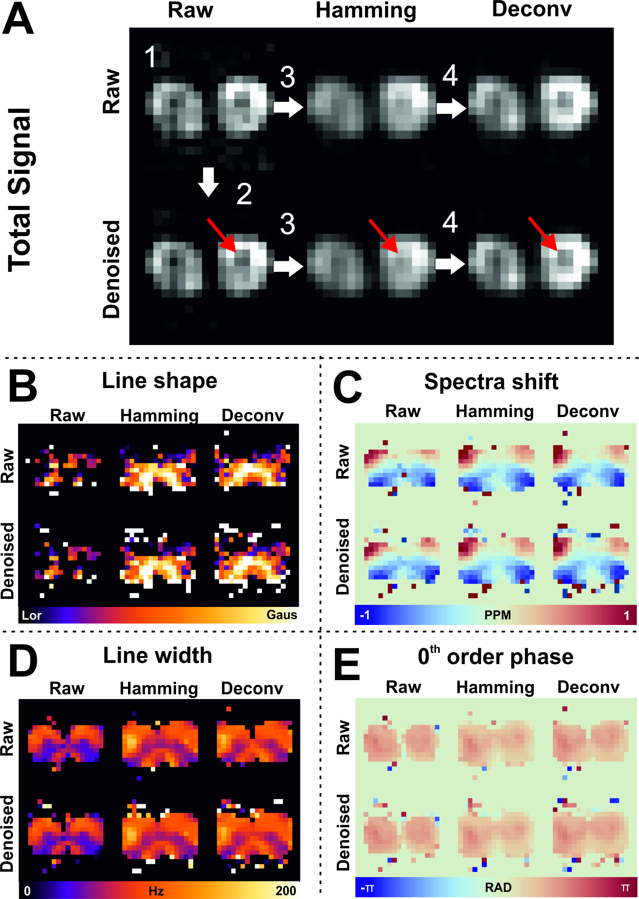
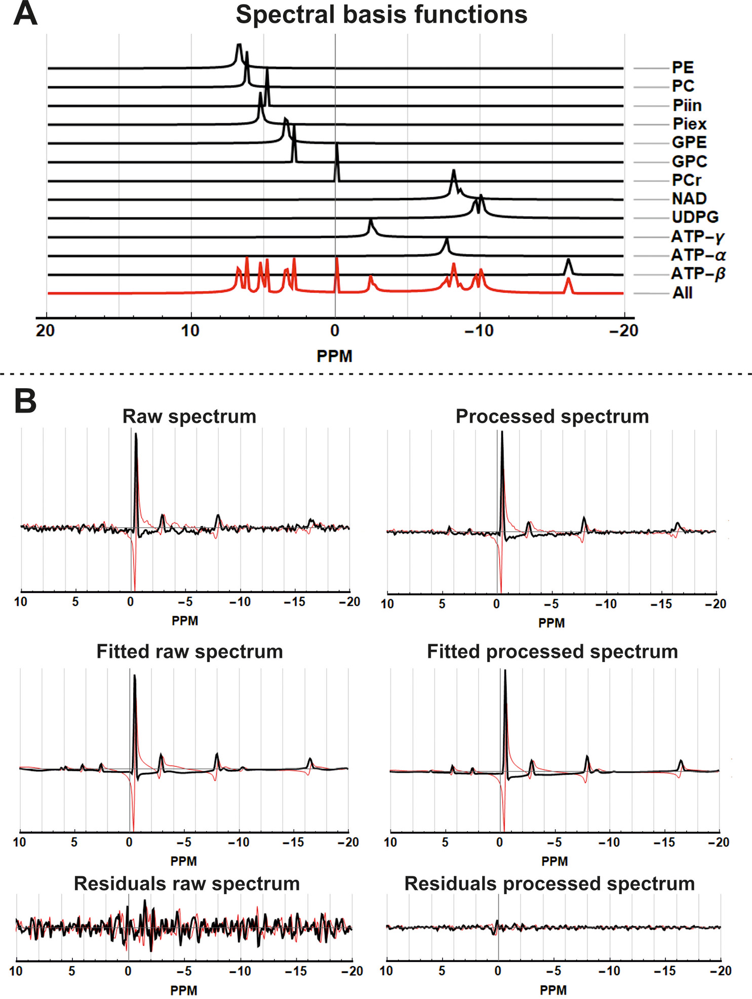
MR experiments were performed on a 7T Philips system with a 31P TX volume transmit coil and a 16-channel receive array (2, 3). The 16 channel 31P receive array also contained 8 TX/RX antennas for 1H imaging. Two experiments were performed: 1) measurement on a phantom consisting of two tubes (diameter 2cm) filled with a 0.1M phosphate solution; 2) in-vivo measurement on the thigh muscles. Data acquisition comprised a 1H localization and a 3D CSI 31P protocol. The CSI acquisition parameters were FOV: 24x32x32 cm3; acq. voxel size: 2x2x6 cm3; NSA: 20; Flip angle 10 degrees; TR/TE: 62/0.45ms; Samples: 256; BW: 4800Hz, scan time 9:48 min.Data reconstruction, processing and fitting was performed using QMRITools for Mathematica (github.com/mfroeling/QMRITools). The raw 16 channel CSI data was reconstructed using SENSE reconstruction where the coil sensitivity maps were estimated by dividing the individual coil data by the sum of squares addition of all coils. Processing of the 3D CSI data comprised three steps as shown in Figure 1: 1) PCA denoising; 2) Hamming apodization; 3) Deconvolution. First the data was denoised using a method commonly used in diffusion imaging, i.e., principal component denoising as first introduced by Veraart et al (4, 5). Next, the data was apodized using a Hamming filter as is commonly done in CSI analysis to reduce Gibbs ringing artifacts with the cost of increasing the point spread function. The last step in the processing was to reduce the point spread function using a 3D iterative steepest decent deconvolution method (6–8). The deconvolution was done on a 2x zero-padded data set, after which the original resolution was restored. Finally, for each processing step all CSI voxels were fitted using basis functions simulated using Hamiltonians similar to Tarquin and LCModel toolboxes for proton spectroscopy (9, 10).
Results
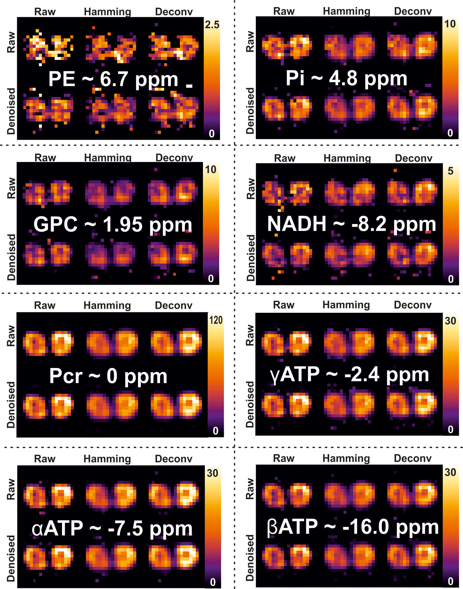
Figure 1 shows the effect of the proposed processing steps on simulated and 3D 31P CSI data of a phantom. PCA denoising removes white noise from the data, after which the Hamming apodization reduces Gibbs ringing and finally the deconvolution restores the point spread function. The effect of denoising on 3D 31P CSI of the upper leg is shown in figure 2, from which it is clear that only noise is removed from the data. Importantly, in figure 2B in the middle column it can be seen that Gibbs ringing artifacts of the PCr peak are revealed after denoising that were not seen in the raw data. Examples of fitted spectum using spectral basis functions are shown in figure 3, where the processed spectra is denoised, Hamming filtered and Deconvolved. The mean fitted line width, line shape, 0th order phase and spectra peak shifts of all metabolites for all processing steps (with and without denoising) are shown in figure 4. The most apparent effect is that Hamming apodization increases the line width and changes the line-shape from Lorentzian to more Gaussian which is only partially corrected by the deconvolution. Finally, the fitted signal amplitudes of 8 metabolites are shown in figure 5. Especially for the low-amplitude signals, such as PE, Pi, GPC and NADH, the beneficial effect of denoising can be seen. In all parameter maps deconvolution restores the signal localization.Discussion and Conclusion
With improved hardware for 31P CSI, such as a dedicated volume transmit coil and high-density receiver arrays on 7T systems, higher spatial coverage of 3D CSI data with improved spatial resolution and SNR can be obtained. In these conditions, processing methods from the imaging domain can be applied successfully to CSI data. In this study we have shown that denoising and deconvolution can enhance 31P CSI data of skeletal muscle, which partially restores the spatial localization when compared to traditional Hamming filtering alone, can increase SNR up to about 2.5-fold and consequently improves spectra fitting.Acknowledgements
No acknowledgement found.References
1. Nagel AM, Laun FB, Weber MA, Matthies C, Semmler W, Schad LR: Sodium MRI using a density-adapted 3D radial acquisition technique. Magn Reson Med 2009; 62:1565–1573.
2. Valkovič L, Dragonu I, Almujayyaz S, et al.: Using a whole-body 31 P birdcage transmit coil and 16-element receive array for human cardiac metabolic imaging at 7T. PLoS One 2017; 12.
3. Löring J, van der Kemp WJM, Almujayyaz S, van Oorschot JWM, Luijten PR, Klomp DWJ: Whole-body radiofrequency coil for 31P MRSI at 7T. NMR Biomed 2016; 29:709–720.
4. Veraart J, Fieremans E, Novikov DS: Diffusion MRI noise mapping using random matrix theory. Magn Reson Med 2016; 76:1582–1593.
5. Veraart J, Novikov DS, Christiaens D, Ades-aron B, Sijbers J, Fieremans E: Denoising of diffusion MRI using random matrix theory. Neuroimage 2016; 142:394–406.
6. Sun PZ: Development of intravoxel inhomogeneity correction for chemical exchange saturation transfer spectral imaging: a high‐resolution field map‐based deconvolution algorithm for magnetic field inhomogeneity correction. Magn Reson Med 2019:mrm.28015.
7. Debnath A, Rai HM, Yadav C, Agarwal A, Bhatia A: Deblurring and Denoising of Magnetic Resonance Images Using Blind Deconvolution Method. Volume 81; 2013.
8. Veraart J, Fieremans E, Jelescu IO, Knoll F, Novikov DS: Gibbs ringing in diffusion MRI. Magn Reson Med 2016; 76:301–314.
9. Provencher SW: Automatic quantitation of localized in vivo 1H spectra with LCModel. NMR Biomed 2001; 14:260–264.
10. Wilson M, Reynolds G, Kauppinen RA, Arvanitis TN, Peet AC: A constrained least-squares approach to the automated quantitation of in vivo 1 H magnetic resonance spectroscopy data . Magn Reson Med 2011; 65:1–12.
Figures