Introduction

²³Na relaxation times in diseased tissue can be altered and relaxation-weighted images can provide additional specific information, e.g. in tumor tissue^1,2. Consequently, several studies have aimed for quantification of the relaxation times^2,3,4. However, these measurements require long acquisition times due to the low in-vivo concentrations and the low NMR sensitivity of sodium. Magnetic Resonance Fingerprinting (MRF) has been shown to be an efficient technique for multi-parametric quantification in ¹H-MRI⁵. Non-steady-state conditions are generated by temporal variations of excitations, gradients and sequence timings, resulting in a unique signal evolution for each combination of relaxation constants. In this work, we present a technique referred as ²³Na-MRF that enables simultaneous quantification of T₁, T_2s^*, T_2l^*, T₂^* and ΔB₀, with automatic differentiation between bi- and monoexponential transverse relaxation.

Methods

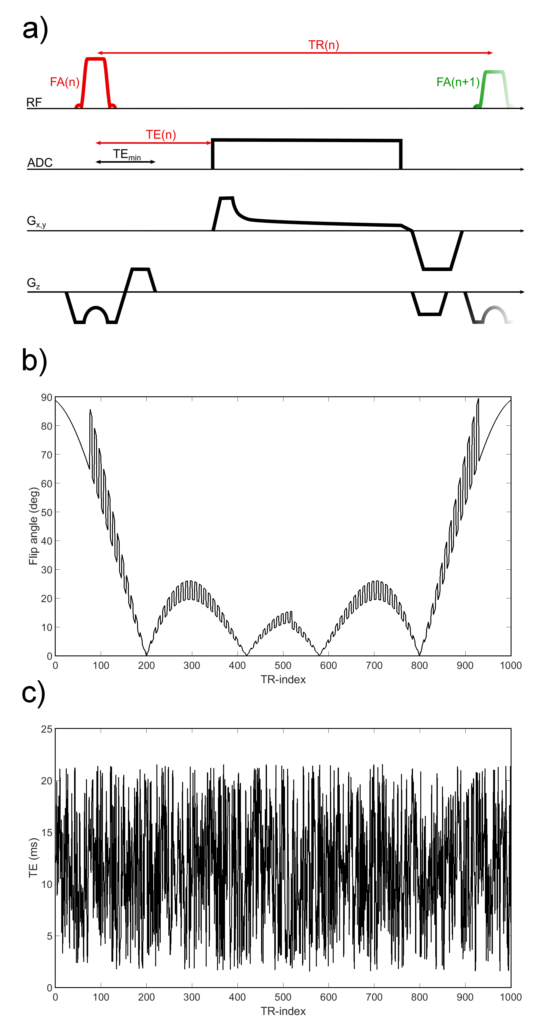
A 2D density-adapted radial spoiled SSFP (FISP) sequence⁶ using VERSE excitation was used for the acquisition of 1000 timeframes with variable flip angle (FA), echo time (TE) and repetition time (TR) patterns. The sequence scheme and the FA pattern are shown in Fig.1. The TE pattern was chosen pseudo randomly between TEmin=1.55ms and 21.55ms (c.f.Fig.1). In each timeframe the smallest possible TR was chosen; consequently, the TR is equal to the TE plus the durations of the gradients, resulting in a TR pattern between 13.34ms and 33.34ms.
For each pulse train, i.e. the measurement of 1 radial spoke in each timeframe, each spoke angle was imcremented by 111.2 degrees relative to the previous one. For a resolution of 2x2x12mm³/4x4x12mm³ 14/7 pulse trains were acquired, resulting in 1000 golden angle-rotated timeframes in k-space containing 14/7 spokes each.
In a first step, adapted Bloch equations were assumed to approximate the system, whereby T_2s^* and T_2l^* correspond to the short and the long transverse relaxation component:
$$\frac{d}{dt}\begin{pmatrix}M_x\\M_y\\M_z\end{pmatrix}=\begin{pmatrix}-\frac{0.6}{T_{2s}^*}-\frac{0.4}{T_{2l}^*}&{\gamma}B_z&-{\gamma}B_y\\-{\gamma}B_z&-\frac{0.6}{T_{2s}^*}-\frac{0.4}{T_{2l}^*}&{\gamma}B_x\\{\gamma}B_y&-{\gamma}B_x&-\frac{1}{T_{1}}\end{pmatrix}\begin{pmatrix}M_x\\M_y\\M_z\end{pmatrix}+\begin{pmatrix}0\\0\\\frac{M_0}{T_1}\end{pmatrix}$$
Monoexponential transverse relaxation was modeled with T₁ and T₂^*=T_2s^*=T_2l^*. Furthermore, deviations from the static field ΔB₀ were considered in both models. A dictionary, needed for reconstruction, was simulated containing each combination in the following parameter space: biexponential: T₁=[20,21,…,70]ms, T_2s^*=[1.0,1.3,…,14.8]ms, T_2l^*=[15,16,…,60]ms, ΔB₀=[-60,-58,…,60]Hz; monoexponential: T₁=[30,31,…,90]ms, T₂^*=[5,6,…,80]ms, ΔB₀=[-60,-58,…,60]Hz. The resulting dictionary, containing both bi- and monoexponential transverse relaxation, was compressed using an SVD compression (rank 12).
Reconstructions were performed using a low rank alternating direction method of multipliers approach⁷. An L2 norm in the wavelet domain was used as spatial regularization (λ_phantom=1*10^-2, λ_invivo=5*10^-2, 40 iterations). The relaxation parameters and ΔB₀ were reconstructed pixelwise by finding the highest scalar product between the pixel signal evolution and all dictionary entries. This automatically determined if the bi- or monoexponential model better describes the measured data in each pixel.
Measurements were performed on a 7T research system (Siemens Healthcare, Germany), using a 30-channel ²³Na coil with additional ¹H channel (Rapid Biomed GmbH, Germany) for in-vivo measurements. Phantom experiments were performed with a single-channel ²³Na birdcage coil with ¹H channel (Rapid Biomed GmbH, Germany).
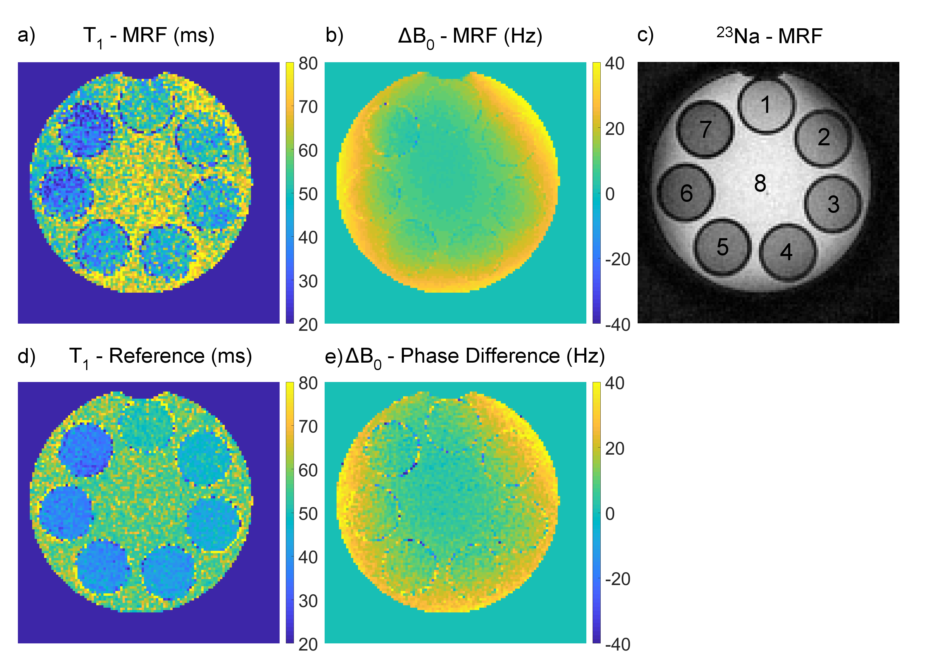
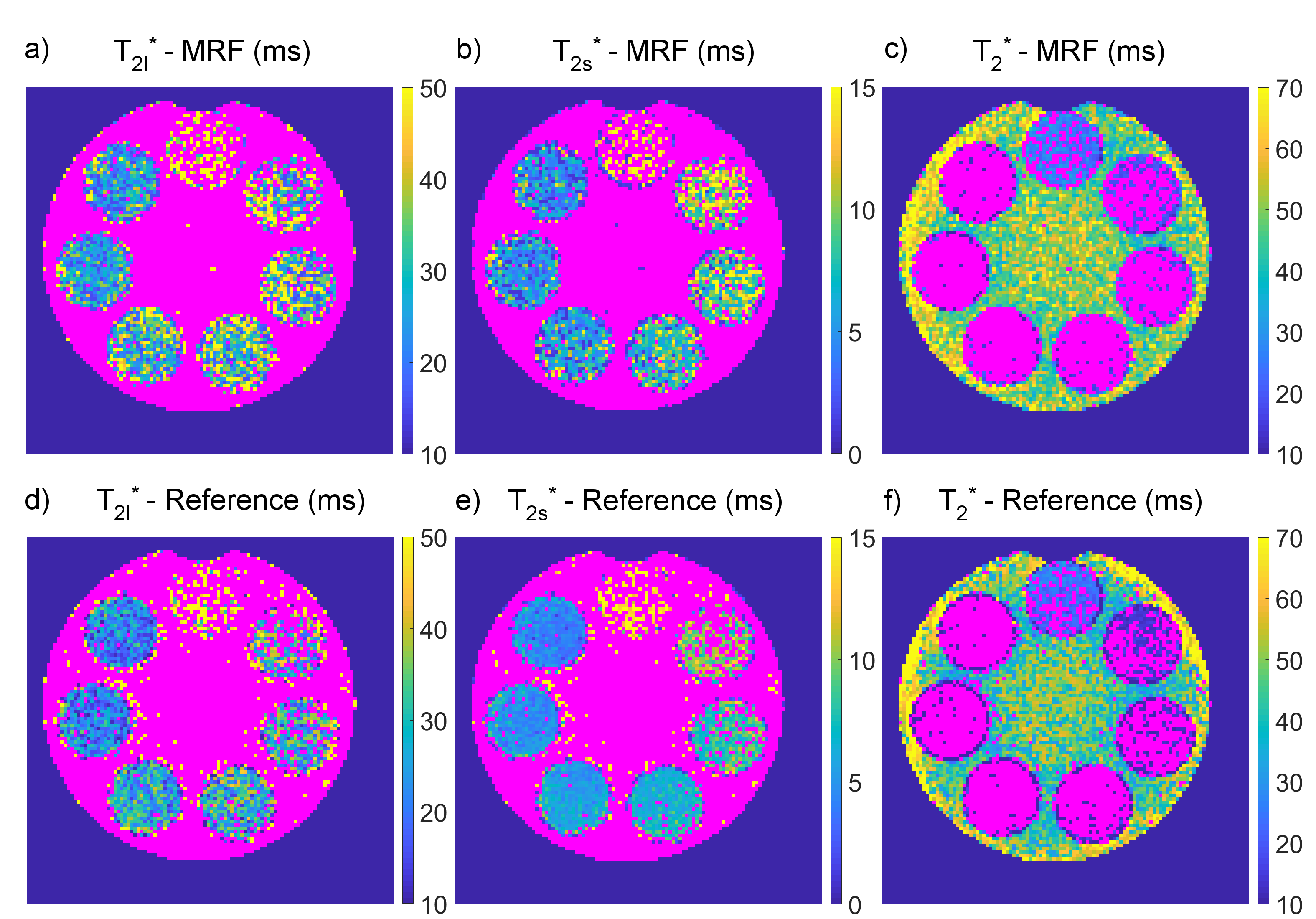
As a reference, the longitudinal relaxation constants were determined by fitting a monoexponential model to the data of a 2D density-adapted radial sequence (TR=300ms,FA=63°,2x2x12mm³,TE=1.34ms,10 averages) with a preceding non-selective inversion pulse and varying inversion times TI=[3.2,10,20,40,70,100,130,160,200,250]ms. The transverse relaxation was determined by fitting both a bi- and monoexponential model to the data acquired with the same sequence without the inversion preparation (TR=200ms,FA=60°,2x2x12mm³,10 averages) and varying TE=[1.24,1.35,2.0,2.5,3,4,5,6,7,9,13,17,23,27,35,40,50,60]ms. Each pixel was assigned to bi- or monoexponential relaxation based on the coefficient of determination (R²) of the fits. Reference maps of ΔB₀ were determined via phase difference between two data sets acquired with the same sequence (TR=25ms,FA=45°,2x2x12mm³,20 averages) with two different echo times (TE1=1.55ms,TE2=6.55ms).
The MRF phantom measurements were performed with a resolution of 2x2x12mm³ (11 averages, 62:16mins measurement time), whereas the in-vivo measurements had a resolution of 4x4x12mm³ (21 averages, 59:26mins measurement time). Mean and standard deviation (SD) were computed in all phantom compartments and in white matter (WM) and cerebrospinal fluid (CSF).

Results

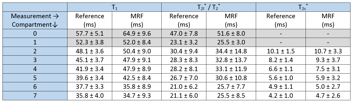
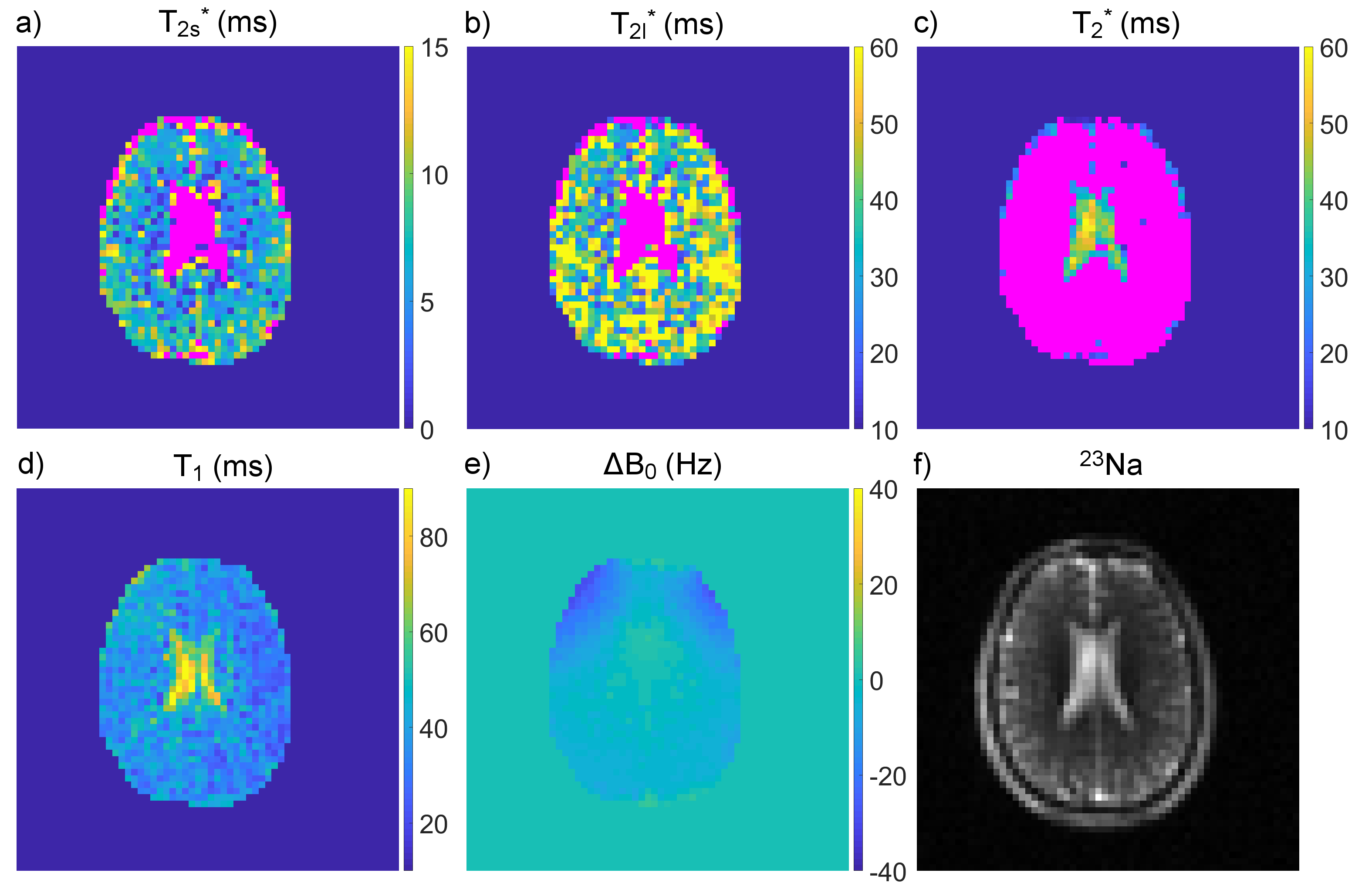
Maps of the relaxation times and ΔB₀ in the phantom are shown in Fig.2 and Fig.3. All mean relaxation times acquired with ²³Na-MRF are in agreement with the reference results within the SD (c.f.Tab.1).
The resulting maps of the in-vivo measurements are displayed in Fig.4. The reconstruction automatically determined biexponential transverse relaxation in brain tissue and monoexponential relaxation in CSF. The following relaxation times, averaged over ROIs, were found for WM: T₁=35.1±8.4ms, T_2l^*=35.2±12.1ms, T_2s^*=5.0±2.5ms. In CSF the values were: T₁=65.5±15.9ms, T₂^*=42.9±8.0ms.

Discussion and Conclusion

This work shows that ²³Na-MRF is highly promising enabling simultaneous measurement of T₁, T_2s^*, T_2l^*, T₂^* and ΔB₀ in-vivo for the first time.
This work is based on adapted Bloch equations as a simplified model that cannot fully describe a spin 3/2 system. This issue could be tackled with irreducible tensor operators⁸. Furthermore, the relaxation models imply a single tissue compartment per pixel. Another improvement could be the use of more sophisticated FA and TE patterns.
Nevertheless, the mean relaxation times in all phantom compartments acquired with ²³Na-MRF are in agreement with the results from the reference method within the error. This demonstrates the potential of ²³Na-MRF for ²³Na relaxometry. Furthermore, the in-vivo results are in good agreement with literature, where the following values have been reported^2,3,4: T_1,CSF=64ms, T_1,WM=37.1ms, T_2,CSF^*=56ms, T_2l,WM^*=25.9-40.9ms, T_2s,WM^*=1.99-6.5ms.

Acknowledgements

No acknowledgement found.