Introduction

The recently proposed DMI is a non-invasive, easy-to-implement and robust metabolic imaging technique ¹. However, acquiring high spatial resolution ²H NMR spectra is often limited due to low SNR inherent to the low metabolite concentrations. Several data processing methods have been proposed to deal with this problem for ¹H MRSI techniques ^{2,3,4,5,6,7,8}. ²H NMR spectra acquired following administration of [6,6-²H₂]-glucose contain only up to 4 non-overlapping peaks. This relative simplicity makes DMI data a good candidate for a machine learning approach. We therefore combine deep learning with ²H MRSI data acquisition to increase the spatial resolution of DMI without compromising spectral quantification.

Methods

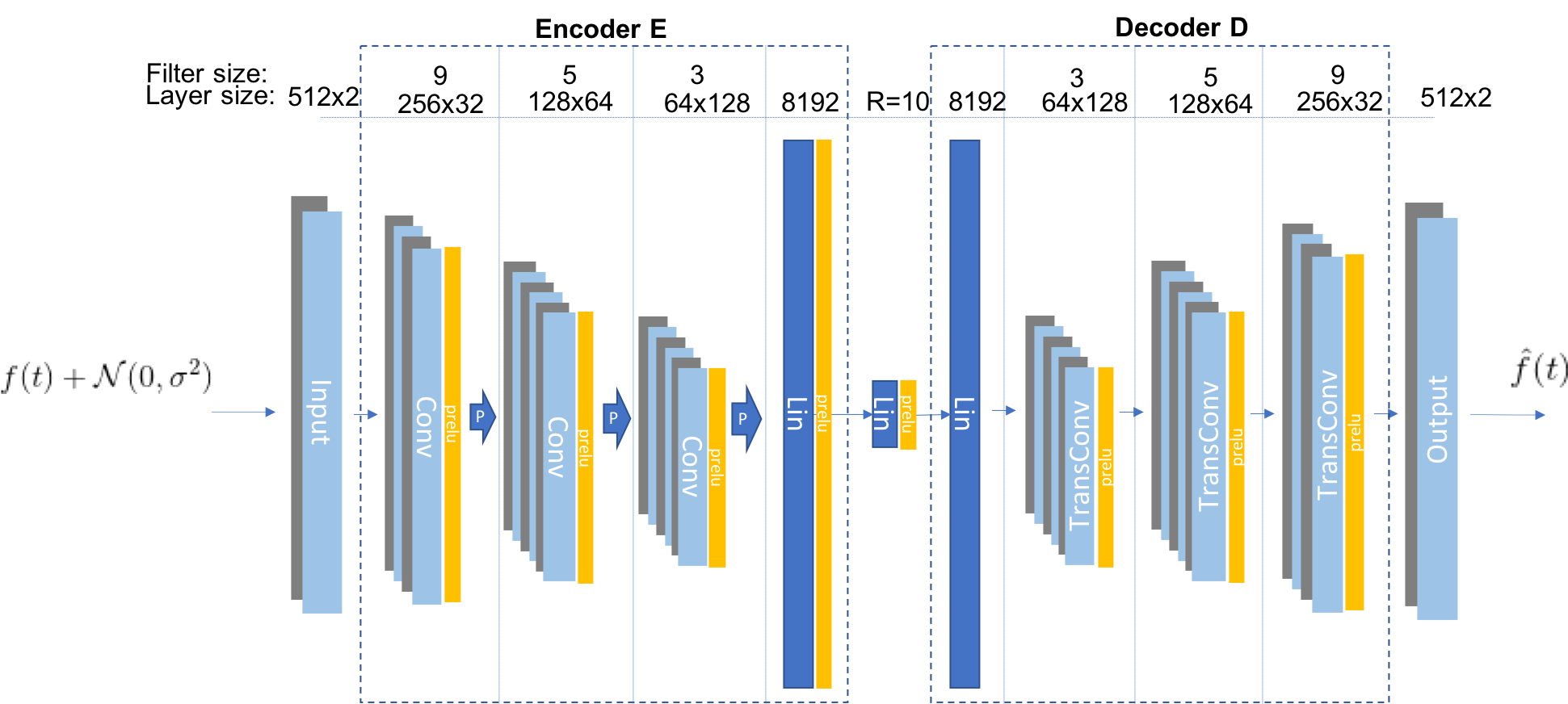
To increase spatial resolution of DMI we relied on a data-driven method using a common architecture in deep learning, autoencoder (AE), and a technique called transfer learning. AE is a type of neural network for learning efficient encodings of high-dimensional input data in an unsupervised manner. Specifically, it minimizes the mean-square-error loss function
$$L=||\mathbf{f}-D(E(\mathbf{f})))||_2$$
by finding the optimal parameterization of the encoder $$$E(\cdot)$$$ and the decoder $$$D(\cdot)$$$. Fig.1 shows the described architecture: a deep convolutional AE. The rationale is based on the notion that 1) compressing a noisy free induction decay (FID) $$$\mathbf{f}$$$ to a low-dimensional representation $$$E(\mathbf{f})$$$ removes insignificant features (noise) and that 2) features of the representation can be pre-determined from synthesized FIDs. The method consists of two steps: decoder-learning and representation-learning. In the decoder-learning step, AE is trained on a large number of synthesized noiseless FIDs (>10k, 80% training and 20% validation) which are generated through the standard FID specification
$$f(t)=\sum^M_{m=1}A_m exp(2\pi i(f_m+\delta f)t)exp(i\phi_m)exp(-\frac{t}{T_m})$$
where the chemical shifts $$$f_m$$$ come from prior knowledge, $$$\delta f$$$ models slight frequency shifts and $$$M$$$ denotes the expected number of distinct metabolites. Amplitudes $$$A_m$$$, lineshape parameters $$$T_m$$$, phases $$$\phi_m$$$ and $$$\delta f$$$ are each randomly generated from a uniform distribution over a reasonable range. After the training process, the decoder learns how to map from the low-dimensional representations to the noiseless FIDs. In the representation-learning step, the encoder is retrained (decoder frozen) on real DMI FIDs to find the representations that give the best reconstruction in terms of mean-squared-error. This is motivated by the idea of transfer learning where the model trained in one domain is used in another. A forward pass through the trained AE plus phase correction gives the final reconstruction. The decoder-learning step is only done once before it can be applied to different datasets with similar metabolic contents to execute the representation-learning step, which takes only ~2min for a 32x32x32 DMI dataset.
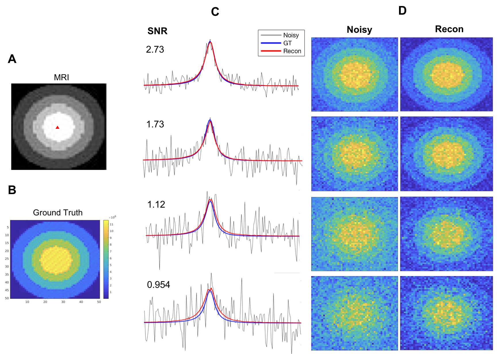
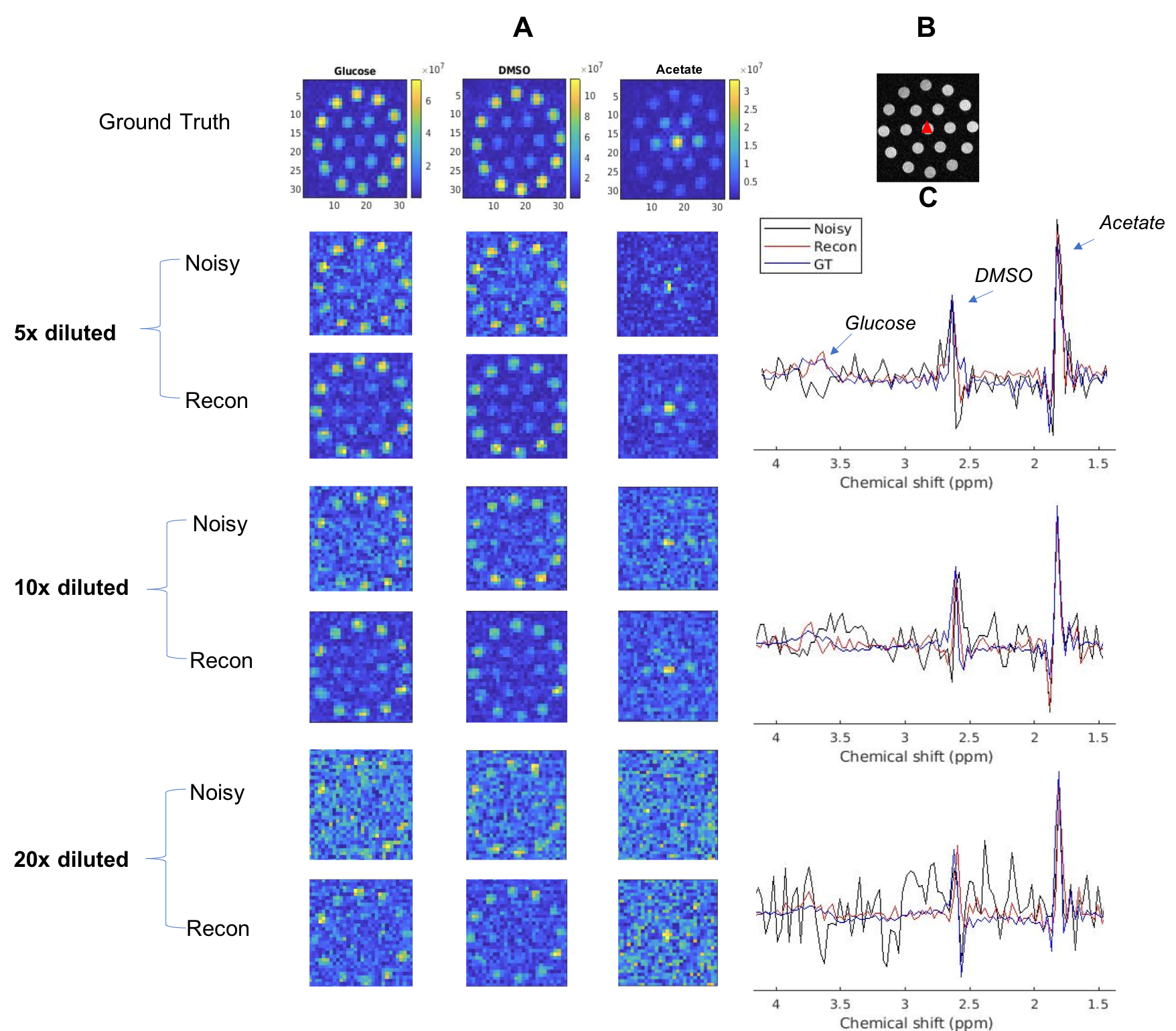
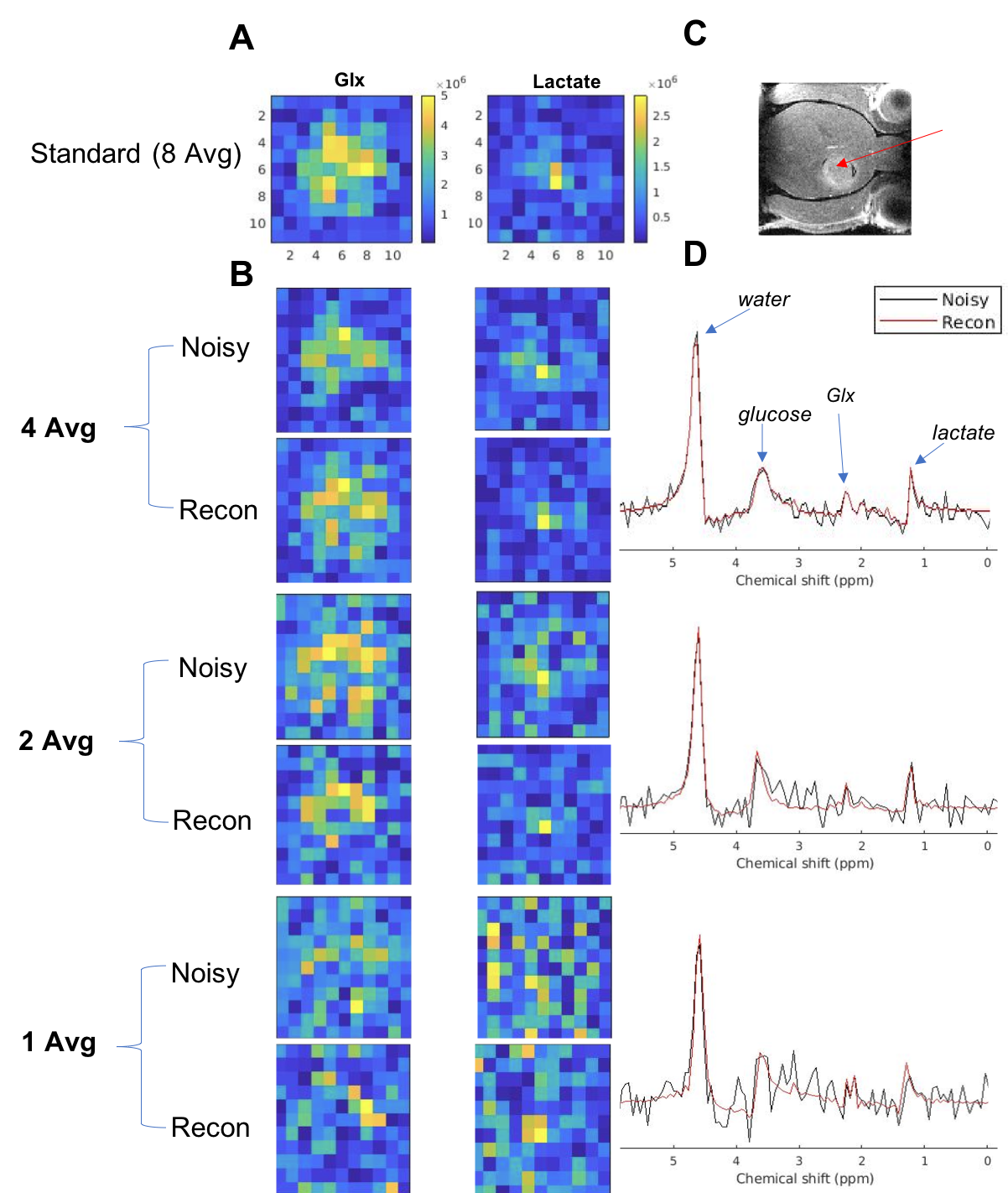
The algorithm's performance is demonstrated on simulated data, phantom data and in vivo data. The simulated experiment verifies the method on ²H NMR spectra containing a peak with Lorentzian lineshape. The phantom was constructed with multiple NMR tubes (Fig.4B) containing solutions of varying concentrations of ²H-labeled glucose, acetate and dimethyl sulfoxide (DMSO). The "ground truth" data were acquired in 1M solutions of the metabolites, and lower SNR DMI datasets were obtained by dilution. DMI data of brain glucose metabolism were acquired in vivo after administration of [6,6-²H₂]-glucose in a Fischer 344 rat implanted with an RG2 brain tumor as described previously ¹. The in vivo DMI data were acquired with 1 to 8 averages, to vary SNR levels.

Results and Discussion

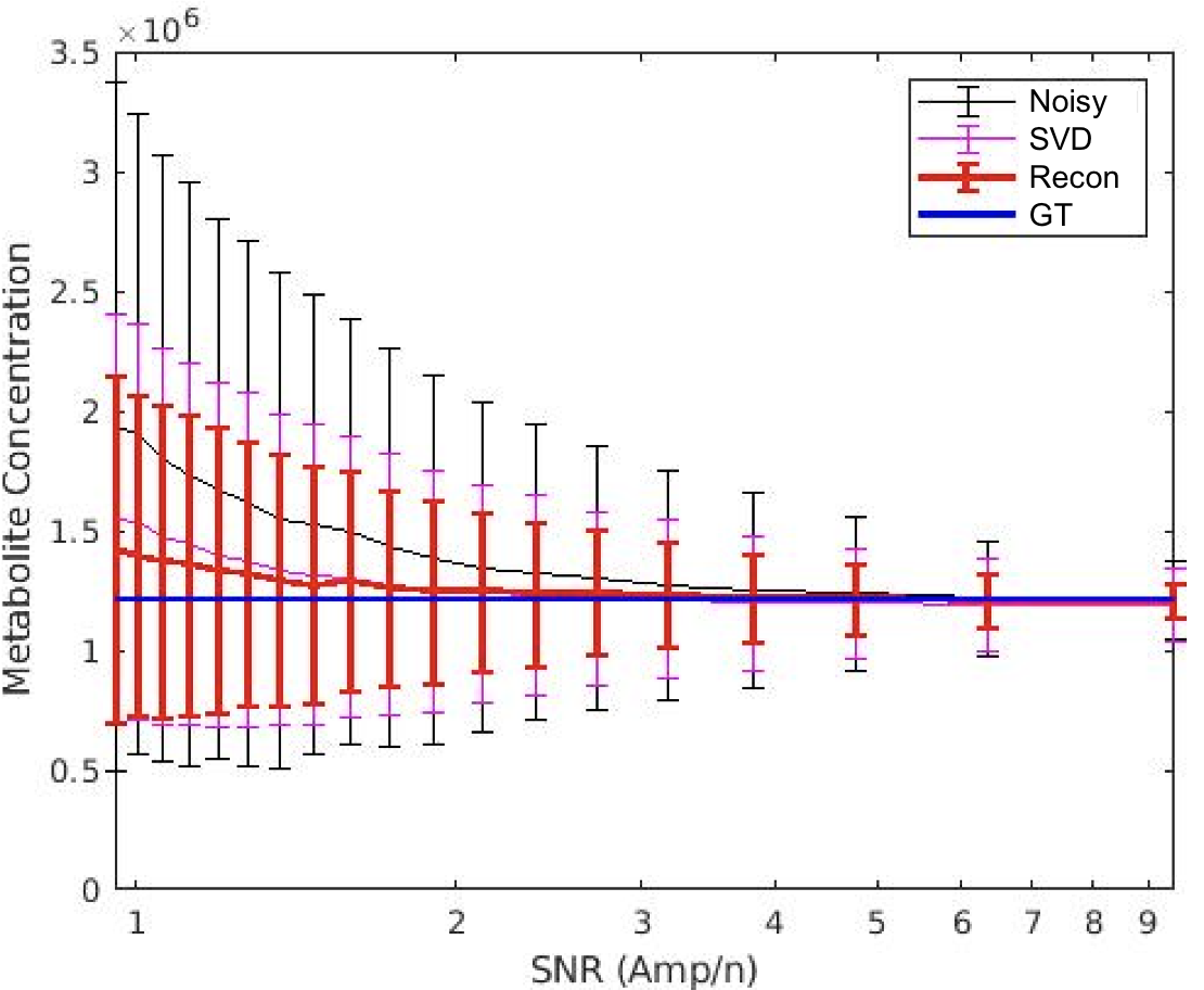
The performance of the algorithm on simulated data indicates that the reconstructed data approach the ground truth, and concentration maps are visually more diagnosable after reconstruction (Fig.2). The method improves the precision of the concentration measurement by 2 to 3 folds compared to the unprocessed data as illustrated by the standard deviation (SD) error bars in Fig.3. The SD of reconstructed data at SNR=2.5 is roughly that of unprocessed data at SNR=6.2. This implies that higher spatial resolution DMI datasets can be acquired (~1.4x higher in each direction) without a penalty in precision of the metabolite concentration estimates. Our newly described method also performed better than standard singular value decomposition (SVD) methods, a technique used in some aspects of previously described de-noising algorithms ^2,6,7,8 (Fig. 3).
The algorithm also improved the appearance of phantom (Fig. 4) and in vivo DMI data (Fig. 5), showing that at least a 2-fold reduction in SNR can be tolerated. A slight reduction in performance is anticipated when using phantom and in vivo DMI data because of magnetic field inhomogeneity and multi-peak spectra phase correction.
In its current installation the described algorithm relies only on the known spectral information. The performance of the method is anticipated to improve further when spatial information is included, quantified magnetic field inhomogeneity (B₀ map) is incorporated, and a more advanced learning methodology is designed.

Conclusion

A novel data-driven method using a deep convolutional autoencoder and transfer learning was implemented to improve the spatial resolution of DMI datasets while maintaining precision in determination of ²H-labeled metabolite concentrations. The algorithm-based reconstruction resulted in a 2-3 folds increase in SNR, which translates to a 40% increase in spatial resolution for DMI without any modification to hardware or data acquisition needed. The technique can be extended to other metabolic imaging techniques (¹H MRSI) by synthesizing different training FIDs.

Acknowledgements

The research is supported by NIH grant R01EB025840, R01CA206180 and R01NS035193.