Introduction

MRI protocols for tumor imaging often require at least 3 different contrasts, including anatomical images such as T1 and T2 weighted, and diffusion-weighted images. In the recent years many attempts have been made to automatically analyze multi-parametric image data^1–5. In particular, convolutional neural network (CNN) analysis has shown great promise in the automatic segmentation of tumor lesions. In this study on head and neck squamous cell carcinoma (HNSCC) patients, multiparametric MRI data are used to train a CNN for tumor and lymph node segmentation. Each 3D MRI contrast served as one input channel to the network. To study robustness against MR image noise, a CNN designed for tumor segmentation was trained and tested on separate data with different SNR levels added to each image retrospectively.

Materials and Methods

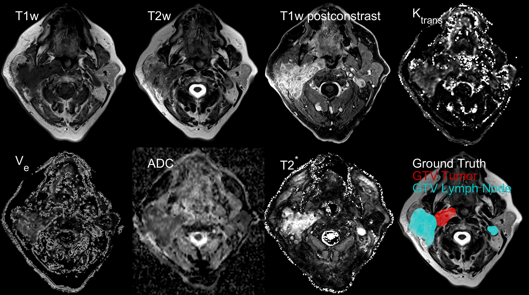
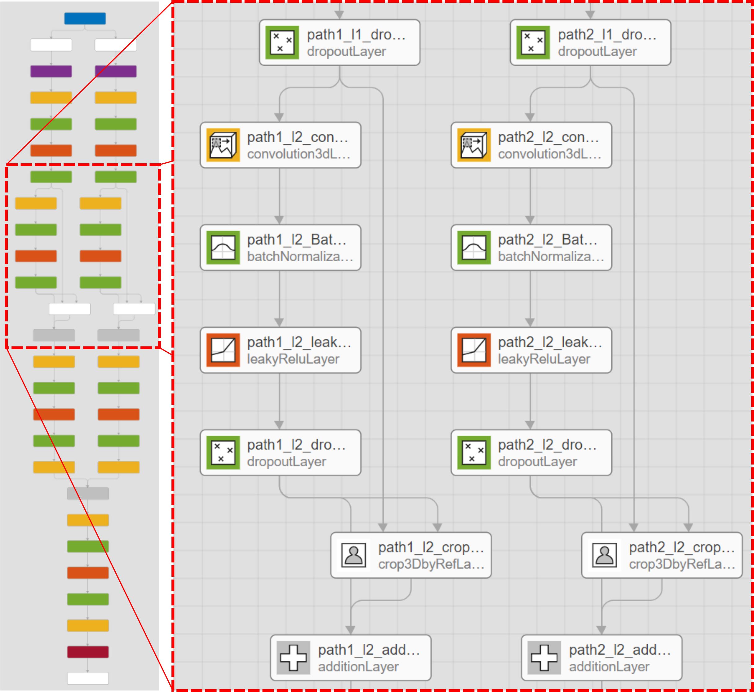
Multiparametric MRI data were taken from a prospective clinical trial in patients suffering from HNSCC. Written informed consent was obtained from each patient. In total, 44 data sets were used including seven channels: pre-contrast T1w and T2w fast Spin Echo, T2* maps, perfusion maps k_trans and v_e from a dynamic contrast-enhanced acquisition, an ADC map acquired from diffusion-weighted data and T1w post-contrast water image (Dixon). All data were acquired on a clinical 3T MRI system (Siemens, Tim® MAGNETOM Trio™). A representative axial slice featuring all contrasts is shown in Fig.1. To process the data, images were normalized to 0.25 mean and standard deviation followed by registration and interpolation to a common resolution of 0.45×0.45×2 mm³. A 3D CNN of the DeepMedic⁵ architecture was trained for the segmentation of gross tumor volume (GTV-T) and lymph node metastases (GTV-LN). Fig.2 shows a minimal example of the network structure that was imported into MATLAB® (Version. 2019a, The MathWorks, Inc.). Network depth, network width and initial learning rate were optimized using a Bayesian optimization scheme⁶ to maximize segmentation performance (training Dice error) within two epochs. The resulting optimized parameters were used to train the full network within 30 epochs on four NVIDIAT4 Tensor Core GPUs. To allow processing of large 3D volumes (Matrix size up to 470×515×37) each image was split into 200 patches of 165×165×9 voxels, resulting in 8800 training images in total. The center location of each patch was chosen randomly with respect to the original image. The probability of the center pixel to be a member of the classes background, GTV-T or GTV-LN was set to 1/3 each to account for class imbalance. Furthermore, a chance of 75% for a random 2D-rotation in the axial plane was added for data augmentation. During the CNN testing phase the complete multiparametric 3D image data of a test patient was segmented. To test the noise robustness, normally distributed noise with different noise amplitudes was added to different data channels . The resulting segmentation performance was subsequently compared to evaluate the noise robustness of the CNN in the various MRI contrasts.

Results

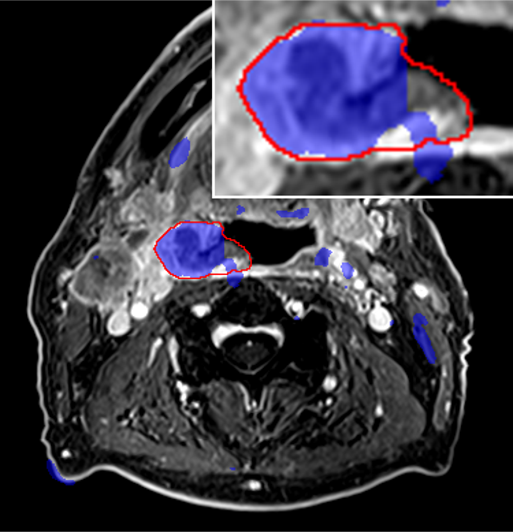
Fig.3 shows the tumor segmentation in the test patient that was not used for CNN training. There is excellent agreement of the tumor borders for a large part of the segmentation (blue) and the ground truth labels (red border). However, many areas of false positives far from the actual tumor region can be found. Fig.4 (top row) shows the evolution of the overall segmentation performance with increasing added noise to each of the input channels. As expected, segmentation performance gradually decreases with increasing noise (i.e., lower SNR). Overall, the CNN still produced good segmentation results at an SNR of 10 on any channel. At very high noise levels (SNR<1) the performance dropped close to 0. The noise sensitivity of the CNN analysis differs depending on the SNR in each input channel (Fig.4 bottom row). At intermediate SNRs (1≤SNR≤ 9) the T1w post-contrast channel was most robust to noise for the segmentation of GTV-T, while k_trans was most robust for GTV-LN.

Discussion and Conclusion

In this study Gaussian noise was added to the input images to resemble the statistics of high SNR magnitude MRI images. As expected, a CNN cannot create a useful segmentation at very low SNR on any single input channel. This indicates that a complete set of input data is always required to create reliable results, and that it might be better to train additional CNNs with fewer input channels in case data with a sufficient quality are missing. Alternatively, replacing input channels by noise in the training phase as means of data augmentation may as well increase robustness to missing or corrupted input data. Therefore other than normal noise distributions, e.g. equally distributed noise, would need to be tested as means of increasing robustness to missing data. Equally distributed noise could better act in masking the original information without adding any additional information. However, this does not resemble the Rician noise statistics commonly found in any MRI image⁷. Fig.4 shows that noise robustness of the trained CNN depends on the input channel and the segmentation target. In accordance with previous results on input channel information content⁸, pre-contrast T1w and T2w input channels showed a high sensitivity to decreasing SNR for both targets (GTV-T & GTV-LN). This implies the need for high image quality on purely anatomical contrasts.

Acknowledgements

This work was partially supported by the Joint Imagin Project (JIP) of the German Consortium for Translational Cancer Research (DKTK).